

MS Excel: Two-Dimensional Lookup (Example #3)
This Excel tutorial explains how to perform a two-dimensional lookup (with screenshots and step-by-step instructions). This is example #3.
Question: I need to find the value on a chart (see below). The only problem is that I can have a quantity value that is not an exact match to a value on the chart. In this case, I need to round down and find the next smaller amount. For example, if I have 51 lbs as a quantity, it should return the value for 50 lbs.
Answer: In effect, what we are trying to do is perform a 2-dimensional lookup in Excel. To find a value in Excel based on both a column and row value, you will need to use both a HLOOKUP function and a MATCH function.
Let's look at an example to see how you would use this function in a worksheet:
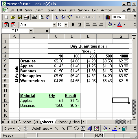
In the spreadsheet above, we have a listing of materials (Oranges, Apples, Bananas, Pineapples, Watermelons) and a listing of quantity columns (50 lbs, 100 lbs, 200 lbs, 500 lbs, 1000 lbs). What we want to do is find the correct value based on a material and quantity combination.
In the first case, we want to find the chart value for 50 lbs of apples. We've entered the following formula into cell D13:
=HLOOKUP(C13, $B$4:$G$9, MATCH(B13, $B$4:$B$9, 0), TRUE)
This formula returns $1.43.
The last parameter on the HLOOKUP function is set to TRUE. This means that if the HLOOKUP does not find an exact match for the quantity, it will look for the next smaller value. (In other words, rounding down)
In the second example, we are looking for the chart value for 1200 lbs of bananas We've entered the following formula into cell D14:
=HLOOKUP(C14, $B$4:$G$9, MATCH(B14, $B$4:$B$9, 0), TRUE)
This formula returns $0.97.
Advertisements