

MS Excel: How to use the TRUNC Function (WS)
This Excel tutorial explains how to use the Excel TRUNC function with syntax and examples.
Description
The Microsoft Excel TRUNC function returns a number truncated to a specified number of digits.
The TRUNC function is a built-in function in Excel that is categorized as a Math/Trig Function. It can be used as a worksheet function (WS) in Excel. As a worksheet function, the TRUNC function can be entered as part of a formula in a cell of a worksheet.
Syntax
The syntax for the TRUNC function in Microsoft Excel is:
TRUNC( number, [digits] )
Parameters or Arguments
- number
- The number to truncate.
- digits
- Optional. It is the number of decimal places to display in the resulting truncated number. If this parameter is omitted, the TRUNC function will assume 0.
Returns
The TRUNC function returns a numeric value.
Applies To
- Excel for Office 365, Excel 2019, Excel 2016, Excel 2013, Excel 2011 for Mac, Excel 2010, Excel 2007, Excel 2003, Excel XP, Excel 2000
Type of Function
- Worksheet function (WS)
Example (as Worksheet Function)
Let's look at some Excel TRUNC function examples and explore how to use the TRUNC function as a worksheet function in Microsoft Excel:
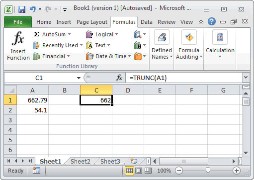
Based on the Excel spreadsheet above, the following TRUNC examples would return:
=TRUNC(A1)
Result: 662

=TRUNC(A1, 0)
Result: 662

=TRUNC(A1, 1)
Result: 662.7

=TRUNC(A2, -1)
Result: 50

=TRUNC(67.891)
Result: 67

=TRUNC(-23.67, 1)
Result: -23.6
Advertisements