Excel: SumProduct Function

In Excel, the SumProduct function multiplies the corresponding items in the arrays and returns the sum of the results.

The syntax for the SumProduct function is:

SumProduct( array1, array2, ... array_n )

array1, array2, ... array_n are the ranges of cells or arrays that you wish to multiply. All arrays must have the same number of rows and columns. You must enter at least 2 arrays and you can have up to 30 arrays.

Applies To:

Excel 2007, Excel 2003, Excel XP, Excel 2000

Note:

If all arrays provided as parameters do not have the same number of rows and columns, the SumProduct function will return the #VALUE! error.

If there are non-numeric values in the arrays, these values are treated as 0's by the SumProduct function.

For example:

Let's take a look at an example:

=SumProduct({1,2;3,4}, {5,6;7,8})

The above example would return 70. The SumProduct calculates these arrays as follows:

=(1*5) + (2*6) + (3*7) + (4*8)

You could also reference ranges in Excel.

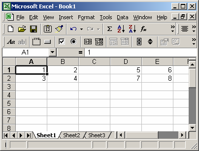
Based on the Excel spreadsheet above, you could enter the following formula:

=SumProduct(A1:B2, D1:E2)

This would also return the value 70.