

MS Excel: How to use the TRANSPOSE Function (WS)
This Excel tutorial explains how to use the Excel TRANSPOSE function with syntax and examples.
Description
The Microsoft Excel TRANSPOSE function returns a transposed range of cells. For example, a horizontal range of cells is returned if a vertical range is entered as a parameter. Or a vertical range of cells is returned if a horizontal range of cells is entered as a parameter.
The TRANSPOSE function is a built-in function in Excel that is categorized as a Lookup/Reference Function. It can be used as a worksheet function (WS) in Excel. As a worksheet function, the TRANSPOSE function can be entered as part of a formula in a cell of a worksheet.
Syntax
The syntax for the TRANSPOSE function in Microsoft Excel is:
TRANSPOSE( range )
Parameters or Arguments
- range
- The range of cells that you want to transpose.
Returns
The TRANSPOSE function returns a transposed range of cells.
Note
- The range value in the TRANSPOSE function must be entered as an array. To enter an array, enter the value and then press Ctrl+Shift+Enter. This will place {} brackets around the formula, indicating that it is an array.
Applies To
- Excel for Office 365, Excel 2019, Excel 2016, Excel 2013, Excel 2011 for Mac, Excel 2010, Excel 2007, Excel 2003, Excel XP, Excel 2000
Type of Function
- Worksheet function (WS)
Example (as Worksheet Function)
Let's look at some Excel TRANSPOSE function examples and explore how to use the TRANSPOSE function as a worksheet function in Microsoft Excel:
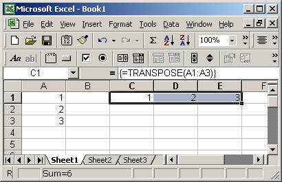
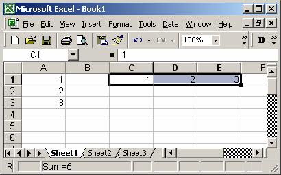
Based on the Excel spreadsheet above:
We've placed values in cells A1, A2, and A3, and we'd like to view these values in cells C1, D1, and E1 (transposed). To do this, you highlight cells C1, D1, and E1, then enter the following formula:
=TRANSPOSE(A1:A3)
Then press Ctrl+Shift+Enter to create an array formula. You will notice that {} brackets will appear around the formula and the values in cells A1, A2, and A3 should now appear in cells C1, D1, and E1.
Frequently Asked Questions
Question: In Microsoft Excel, isn't it easier to use the Paste Special transpose option to do the same?
Answer: Yes, if you ONLY want to perform a one-time paste of the values, you can do the following:
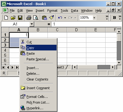
Highlight the cells that you want to copy. In this example, we've highlighted cells A1:A3. Then right-click and select Copy from the popup menu.
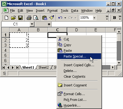
Then right-click on the cell where you'd like to paste the values and select Paste Special from the popup menu.
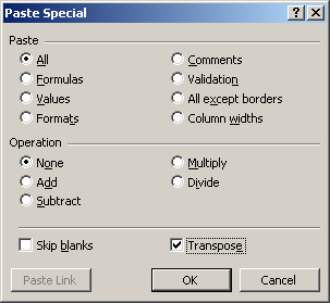
Then select the TRANSPOSE checkbox and click on the OK button.
Now when you return to your spreadsheet, you'll see that the values have been copied and transposed.
Advertisements