

MS Excel: How to use the DSUM Function (WS)
This Excel tutorial explains how to use the Excel DSUM function with syntax and examples.
Description
The Microsoft Excel DSUM function sums the numbers in a column or database that meets a given criteria.
The DSUM function is a built-in function in Excel that is categorized as a Database Function. It can be used as a worksheet function (WS) in Excel. As a worksheet function, the DSUM function can be entered as part of a formula in a cell of a worksheet.
Syntax
The syntax for the DSUM function in Microsoft Excel is:
DSUM( range, field, criteria )
Parameters or Arguments
- range
- The range of cells that you want to apply the criteria against.
- field
- The column to sum the values. You can either specify the numerical position of the column in the list or the column label in double quotation marks.
- criteria
- The range of cells that contains your criteria.
Returns
The DSUM function returns a numeric value.
Applies To
- Excel for Office 365, Excel 2019, Excel 2016, Excel 2013, Excel 2011 for Mac, Excel 2010, Excel 2007, Excel 2003, Excel XP, Excel 2000
Type of Function
- Worksheet function (WS)
Example (as Worksheet Function)
Let's look at some Excel DSUM function examples and explore how to use the DSUM function as a worksheet function in Microsoft Excel:
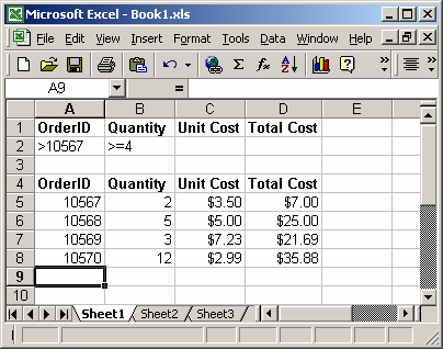
Based on the Excel spreadsheet above, the following DSUM examples would return:
=DSUM(A4:D8, "Unit Cost", A1:B2)
Result: 7.99
Let's quickly explain why the DSUM function returns 7.99 in this example. The criteria for the DSUM calculation is found in cells A1:B2. This means that only those records where the order number is greater than 10567 and Quantity is greater than equal to 4 will be included in the sum calculations.
So in the example above, only rows 6 and 8 meet those conditions. As a result, the DSUM adds together the Unit Cost values in only rows 6 and 8 to return 7.99 (5.00 + 2.99).
Here are some more examples of the DSUM function:
=DSUM(A4:D8, 3, A1:B2)
Result: 7.99

=DSUM(A4:D8, "Quantity", A1:A2)
Result: 20

=DSUM(A4:D8, 2, A1:A2)
Result: 20
Using Named Ranges
You can also use a named range in the DSUM function. A named range is a descriptive name for a collection of cells or range in a worksheet. If you are unsure of how to setup a named range in your spreadsheet, read our tutorial on Adding a Named Range.
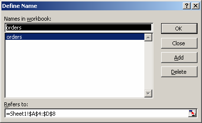
For example, we've created a named range called orders that refers to Sheet1!$A$4:$D$8.
Then we've entered the following data in Excel:
Based on the Excel spreadsheet above, the following DSUM examples would return:
=DSUM(orders, "Total Cost", A1:B2)
Result: 60.88

=DSUM(orders, 4, A1:B2)
Result: 60.88
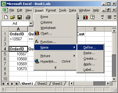
To view named ranges: Under the Insert menu, select Name > Define.
Advertisements