

MS Excel: How to use the MATCH Function (WS)
This Excel tutorial explains how to use the Excel MATCH function with syntax and examples.
Description
The Microsoft Excel MATCH function searches for a value in an array and returns the relative position of that item.
The MATCH function is a built-in function in Excel that is categorized as a Lookup/Reference Function. It can be used as a worksheet function (WS) in Excel. As a worksheet function, the MATCH function can be entered as part of a formula in a cell of a worksheet.
If you want to follow along with this tutorial, download the example spreadsheet.
Syntax
The syntax for the MATCH function in Microsoft Excel is:
MATCH( value, array, [match_type] )
Parameters or Arguments
- value
- The value to search for in the array.
- array
- A range of cells that contains the value that you are searching for.
- match_type
Optional. It the type of match that the function will perform. The possible values are:
match_type Explanation 1 (default) The MATCH function will find the largest value that is less than or equal to value. You should be sure to sort your array in ascending order. If the match_type parameter is omitted, it assumes a match_type of 1.
0 The MATCH function will find the first value that is equal to value. The array can be sorted in any order. -1 The MATCH function will find the smallest value that is greater than or equal to value. You should be sure to sort your array in descending order.
Returns
The MATCH function returns a numeric value.
If the MATCH function does not find a match, it will return a #N/A error.
Note
- The MATCH function does not distinguish between upper and lowercase when searching for a match.
-
If the match_type parameter is 0 and the value is a text value, then you can use wildcards in the value parameter.
Wild card Explanation * matches any sequence of characters ? matches any single character
Applies To
- Excel for Office 365, Excel 2019, Excel 2016, Excel 2013, Excel 2011 for Mac, Excel 2010, Excel 2007, Excel 2003, Excel XP, Excel 2000
Type of Function
- Worksheet function (WS)
Example (as Worksheet Function)
Let's look at some Excel MATCH function examples and explore how to use the MATCH function as a worksheet function in Microsoft Excel:
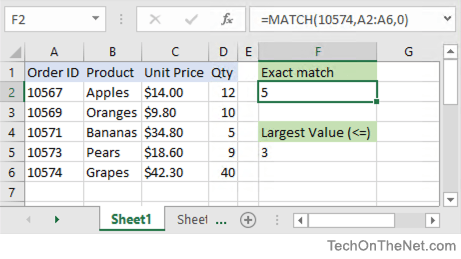
Based on the Excel spreadsheet above, the following MATCH examples would return:
=MATCH(10574,A2:A6,0)
Result: 5     (it matches on 10574)

=MATCH(10572,A2:A6,1)
Result: 3     (it matches on 10571 since the match_type parameter is set to 1)

=MATCH(10572,A2:A6)
Result: 3     (it matches on 10571 since the match_type parameter has been omitted and will default to 1)

=MATCH(10572,A2:A6,0)
Result: #N/A  (it doesn't find a match since the match_type parameter is set to 0)

=MATCH(10573,A2:A6,1)
Result: 4

=MATCH(10573,A2:A6,0)
Result: 4
Let's look at how we can use wild cards in the MATCH function.
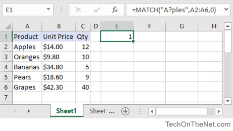
Based on the Excel spreadsheet above, the following MATCH examples would return:
=MATCH("A?ples", A2:A6, 0)
Result: 1

=MATCH("O*s", A2:A6, 0)
Result: 2

=MATCH("O?s", A2:A6, 0)
Result: #N/A
Frequently Asked Questions
Question: In Microsoft Excel, I tried this MATCH formula but it did not work:
=IF(MATCH(B94,Overview!D$54:D$96),"FS","Bulk")
I was hoping for an easier formula than this:
=IF(OR(B94=Overview!D$54,B94=Overview!D55,B94=Overview!D56, {etc thru D96} ),"FS","Bulk")
Answer: When you are using the MATCH function, you need to be aware of a few things.
First, you need to consider whether your array is sorted in a particular order (ie: ascending order, descending order, or no order). Since we are looking for an exact match and we don't know if the array is sorted, we want to make sure that the match_type parameter in the MATCH function is set to 0. This will find a match regardless of the sort order.
Second, we know that the MATCH function will return an #N/A error when a match is not found, so we will want to use the ISERROR function to check for the #N/A error.
So based on these 2 additional considerations, we would want to modify your original formula as follows:
=IF(ISERROR(MATCH(B94,Overview!D$54:D$96,0))=FALSE,"FS","Bulk")
This would check for an exact match in the D54:D96 array on the Overview sheet and return "FS" if a match is found. Otherwise, it would return "Bulk" if no match is found.
Question:I have a question about how to nest a MATCH function within the INDEX function. The question is:
I want to create a formula using the MATCH function nested within the INDEX function to retrieve the Class that was selected (by the x) in E4:F10. The MATCH function should find the row where the x is located and should be used within the INDEX function to retrieve the associated Class value from the same row within F4:F10.
Answer:We can use the MATCH function to find the row position in the range E4:E10 to find the row where "x" is located. We then embed this MATCH function within the INDEX function to return the corresponding value in the range F4:$10 as follow:
=INDEX($F$4:$F$10, MATCH("x",$E$4:$E$10))
In this example, we are searching for the value "x" within the range E4:E10. When the value of "x" is found, it will return the corresponding value from F4:F10.
Advertisements