

MS Excel: How to use the COUNTIFS Function (WS)
This Excel tutorial explains how to use the Excel COUNTIFS function with syntax and examples.
Description
The Microsoft Excel COUNTIFS function counts the number of cells in a range, that meets a single or multiple criteria.
The COUNTIFS function is a built-in function in Excel that is categorized as a Statistical Function. It can be used as a worksheet function (WS) in Excel. As a worksheet function, the COUNTIFS function can be entered as part of a formula in a cell of a worksheet.
If you want to follow along with this tutorial, download the example spreadsheet.
Syntax
The syntax for the COUNTIFS function in Microsoft Excel is:
COUNTIFS( range1, criteria1, [range2, criteria2, ... range_n, criteria_n] )
Parameters or Arguments
- range1
- The range of cells that you want to apply criteria1 against.
- criteria1
- The criteria used to determine which cells to count. criteria1 is applied against range1.
- range2, ... range_n
- Optional. It is the range of cells that you want to apply criteria2, ... criteria_n against. There can be up to 127 ranges.
- criteria2, ... criteria_n
- Optional. It is used to determine which cells to count. criteria2 is applied against range2, criteria3 is applied against range3, and so on. There can be up to 127 criteria.
Returns
The COUNTIFS function returns a numeric value.
Applies To
- Excel for Office 365, Excel 2019, Excel 2016, Excel 2013, Excel 2011 for Mac, Excel 2010, Excel 2007
Type of Function
- Worksheet function (WS)
Example (as Worksheet Function)
Let's look at some Excel COUNTIFS function examples and explore how to use the COUNTIFS function as a worksheet function in Microsoft Excel:
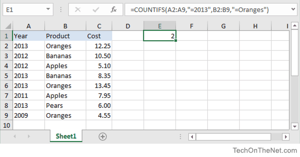
Based on the Excel spreadsheet above, the following COUNTIFS examples would return:
=COUNTIFS(A2:A9,"=2013")
Result: 4   'Applies 1 criteria

=COUNTIFS(A2:A9,"=2013",B2:B9,"=Oranges")
Result: 2   'Applies 2 criteria

=COUNTIFS(A2:A9,">=2009",B2:B9,"=Oranges", A2:A9,"<=2012")
Result: 1   'Applies 3 criteria

=COUNTIFS(A2:A9,">=2009",B2:B9,"=B*")
Result: 2   'Uses the * wildcard to match on all products that start with B

=COUNTIFS(A2:A9,">=2009",B2:B9,"=B?nanas")
Result: 2   'Uses the ? wildcard to match on a single character, ie: Bananas, Benanas, Binanas, Bonanas, and so on
Using Named Ranges
You can also use a named range in the COUNTIFS function. A named range is a descriptive name for a collection of cells or range in a worksheet. If you are unsure of how to setup a named range in your spreadsheet, read our tutorial on Adding a Named Range.
For example, we've created a named range called products that refers to the range B2:B9 in Sheet 1.
Then we've entered the following data in Excel:
Based on the Excel spreadsheet above:
=COUNTIFS(products,"=Apples",A2:A9,">2010")
Result: 2

=COUNTIFS(products,"=Oranges",A2:A9,"<2014")
Result: 3
To view named ranges: Select the Formulas tab in the toolbar at the top of the screen. Then in the Defined Names group, click on the Defined Names drop-down and select Name Manager.
The Name Manager window should now appear.
Advertisements