

MS Excel: How to use the INDEX Function (WS)
This Excel tutorial explains how to use the Excel INDEX function with syntax and examples.
Description
The Microsoft Excel INDEX function returns a value in a table based on the intersection of a row and column position within that table. The first row in the table is row 1 and the first column in the table is column 1.
The INDEX function is a built-in function in Excel that is categorized as a Lookup/Reference Function. It can be used as a worksheet function (WS) in Excel. As a worksheet function, the INDEX function can be entered as part of a formula in a cell of a worksheet.
If you want to follow along with this tutorial, download the example spreadsheet.
Syntax
The syntax for the INDEX function in Microsoft Excel is:
INDEX( table, row_number, column_number )
Parameters or Arguments
- table
- A range of cells that contains the table of data.
- row_number
- The row position in the table where the value you want to lookup is located. This is the relative row position in the table and not the actual row number in the worksheet.
- column_number
- The column position in the table where the value you want to lookup is located. This is the relative column position in the table and not the actual column number in the worksheet.
Returns
The INDEX function returns any datatype such as a string, numeric, date, etc.
Applies To
- Excel for Office 365, Excel 2019, Excel 2016, Excel 2013, Excel 2011 for Mac, Excel 2010, Excel 2007, Excel 2003, Excel XP, Excel 2000
Type of Function
- Worksheet function (WS)
Example (as Worksheet Function)
Let's explore how to use INDEX as a worksheet function in Microsoft Excel.
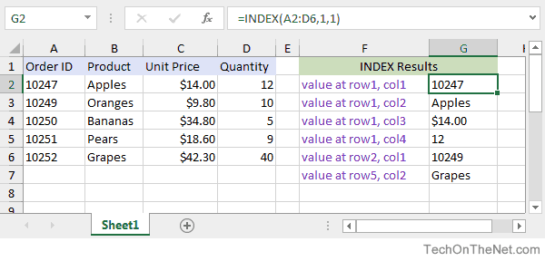
Based on the Excel spreadsheet above, the following INDEX examples would return:
=INDEX(A2:D6,1,1)
Result: 10247     'Intersection of row1 and col1 (cell A2)

=INDEX(A2:D6,1,2)
Result: "Apples"  'Intersection of row1 and col2 (cell B2)

=INDEX(A2:D6,1,3)
Result: $14.00    'Intersection of row1 and col3 (cell C2)

=INDEX(A2:D6,1,4)
Result: 12        'Intersection of row1 and col4 (cell D2)

=INDEX(A2:D6,2,1)
Result: 10249     'Intersection of row2 and col1 (cell A3)

=INDEX(A2:D6,5,2)
Result: Grapes    'Intersection of row5 and col2 (cell B6)
Now, let's look at the example =INDEX(A2:D6,1,1) that returns a value of 10247 and take a closer look why.
First Parameter
The first parameter in the INDEX function is the table or the source of data where the lookup should be performed.
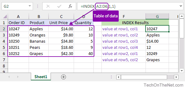
In this example, the first parameter is A2:D6 which defines the range of cells that contains the data.
Second Parameter
The second parameter is the row number used to determine the intersection location in the table. A value of 1 indicates the first row in the table, a value of 2 is the second row, and so on.
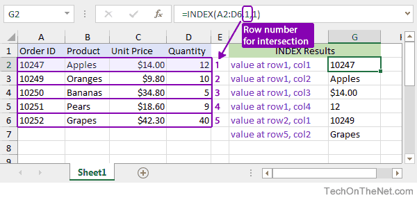
In this example, the second parameter is 1 so we know that our intersection will occur in the first row in the table.
Third Parameter
The third parameter is the column number used to determine the intersection location in the table. A value of 1 indicates the first column in the table, a value of 2 is the second column, and so on.
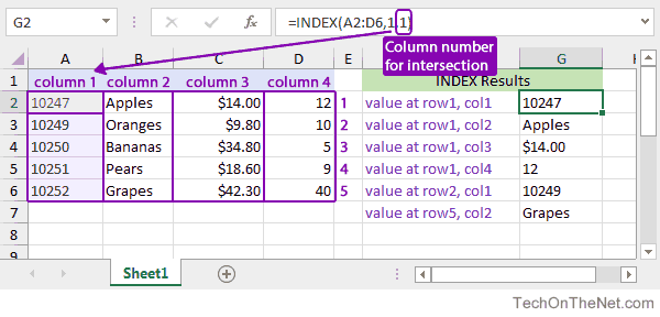
In this example, the third parameter is 1 so we know that our intersection will occur in the first column in the table.
Since we now have our row and column values, we know that we are looking for the intersection of row1 and col1 in the table of data. This makes the intersection point occur at cell A2 in the table so the INDEX function will return the value 10247.
Frequently Asked Questions
If you want to find out what others have asked about the INDEX function, go to our Frequently Asked Questions.
Advertisements