

MS Excel: How to use the Nested IF Functions (WS)
This Excel tutorial explains how to nest the Excel IF function with syntax and examples.
Description
The IF function is a built-in function in Excel that is categorized as a Logical Function. It can be used as a worksheet function (WS) in Excel. As a worksheet function, the IF function can be entered as part of a formula in a cell of a worksheet.
It is possible to nest multiple IF functions within one Excel formula. You can nest up to 7 IF functions to create a complex IF THEN ELSE statement.
Syntax
The syntax for the nesting the IF function is:
IF( condition1, value_if_true1, IF( condition2, value_if_true2, value_if_false2 ))
This would be equivalent to the following IF THEN ELSE statement:
IF condition1 THEN
   value_if_true1
ELSEIF condition2 THEN
   value_if_true2
ELSE
   value_if_false2
END IF
Parameters or Arguments
- condition
- The value that you want to test.
- value_if_true
- The value that is returned if condition evaluates to TRUE.
- value_if_false
- The value that is return if condition evaluates to FALSE.
Note
- This Nested IF function syntax demonstrates how to nest two IF functions. You can nest up to 7 IF functions.
Applies To
- Excel for Office 365, Excel 2019, Excel 2016, Excel 2013, Excel 2011 for Mac, Excel 2010, Excel 2007, Excel 2003, Excel XP, Excel 2000
Type of Function
- Worksheet function (WS)
Example (as Worksheet Function)
Let's look at an example to see how you would use a nested IF and explore how to use the nested IF function as a worksheet function in Microsoft Excel:
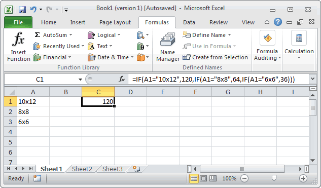
Based on the Excel spreadsheet above, the following Nested IF examples would return:
=IF(A1="10x12",120,IF(A1="8x8",64,IF(A1="6x6",36)))
Result: 120

=IF(A2="10x12",120,IF(A2="8x8",64,IF(A2="6x6",36)))
Result: 64

=IF(A3="10x12",120,IF(A3="8x8",64,IF(A3="6x6",36)))
Result: 36
TIP: When nesting multiple IF functions, DO NOT start the second IF function with = sign.
Incorrect formula:
=IF(A1=2,"Hello",=IF(A1=3,"Goodbye",0))
Correct formula
=IF(A1=2,"Hello",IF(A1=3,"Goodbye",0))
Frequently Asked Questions
Question: In Microsoft Excel, I need to write a formula that works this way:
If (cell A1) is less than 20, then multiply by 1,
If it is greater than or equal to 20 but less than 50, then multiply by 2
If its is greater than or equal to 50 and less than 100, then multiply by 3
And if it is great or equal to than 100, then multiply by 4
Answer: You can write a nested IF statement to handle this. For example:
=IF(A1<20, A1*1, IF(A1<50, A1*2, IF(A1<100, A1*3, A1*4)))
Question:In Excel, I need a formula in cell C5 that does the following:
IF A1+B1 <= 4, return $20
IF A1+B1 > 4 but <= 9, return $35
IF A1+B1 > 9 but <= 14, return $50
IF A1+B1 > 15, return $75
Answer:In cell C5, you can write a nested IF statement that uses the AND function as follows:
=IF((A1+B1)<=4,20,IF(AND((A1+B1)>4,(A1+B1)<=9),35,IF(AND((A1+B1)>9,(A1+B1)<=14),50,75)))
Question: In Microsoft Excel, I need a formula for the following:
IF cell A1= PRADIP then value will be 100
IF cell A1= PRAVIN then value will be 200
IF cell A1= PARTHA then value will be 300
IF cell A1= PAVAN then value will be 400
Answer: You can write an IF statement as follows:
=IF(A1="PRADIP",100,IF(A1="PRAVIN",200,IF(A1="PARTHA",300,IF(A1="PAVAN",400,""))))
Question: In Microsoft Excel, I want to calculate following using an "if" formula:
if A1<100,000 then A1*.1% but minimum 25
and if A1>1,000,000 then A1*.01% but maximum 5000
Answer: You can write a nested IF statement that uses the MAX function and the MIN function as follows:
=IF(A1<100000,MAX(25,A1*0.1%),IF(A1>1000000,MIN(5000,A1*0.01%),""))
Question:I have Excel 2000. If cell A2 is greater than or equal to 0 then add to C1. If cell B2 is greater than or equal to 0 then subtract from C1. If both A2 and B2 are blank then equals C1. Can you help me with the IF function on this one?
Answer: You can write a nested IF statement that uses the AND function and the ISBLANK function as follows:
=IF(AND(ISBLANK(A2)=FALSE,A2>=0),C1+A2, IF(AND(ISBLANK(B2)=FALSE,B2>=0),C1-B2, IF(AND(ISBLANK(A2)=TRUE, ISBLANK(B2)=TRUE),C1,"")))
Question:How would I write this equation in Excel? If D12<=0 then D12*L12, If D12 is > 0 but <=600 then D12*F12, If D12 is >600 then ((600*F12)+((D12-600)*E12))
Answer: You can write a nested IF statement as follows:
=IF(D12<=0,D12*L12,IF(D12>600,((600*F12)+((D12-600)*E12)),D12*F12))
Question:I have read your piece on nested IFs in Excel, but I still cannot work out what is wrong with my formula please could you help? Here is what I have:
=IF(63<=A2<80,1,IF(80<=A2<95,2,IF(A2=>95,3,0)))
Answer: The simplest way to write your nested IF statement based on the logic you describe above is:
=IF(A2>=95,3,IF(A2>=80,2,IF(A2>=63,1,0)))
This formula will do the following:
If A2 >= 95, the formula will return 3 (first IF function)
If A2 < 95 and A2 >= 80, the formula will return 2 (second IF function)
If A2 < 80 and A2 >= 63, the formula will return 1 (third IF function)
If A2 < 63, the formula will return 0
Question:I'm very new to the Excel world, and I'm trying to figure out how to set up the proper formula for an If/then cell.
What I'm trying for is:
If B2's value is 1 to 5, then multiply E2 by .77
If B2's value is 6 to 10, then multiply E2 by .735
If B2's value is 11 to 19, then multiply E2 by .7
If B2's value is 20 to 29, then multiply E2 by .675
If B2's value is 30 to 39, then multiply E2 by .65
I've tried a few different things thinking I was on the right track based on the IF, and AND function tutorials here, but I can't seem to get it right.
Answer:To write your IF formula, you need to nest multiple IF functions together in combination with the AND function.
The following formula should work for what you are trying to do:
=IF(AND(B2>=1, B2<=5), E2*0.77, IF(AND(B2>=6, B2<=10), E2*0.735, IF(AND(B2>=11, B2<=19), E2*0.7, IF(AND(B2>=20, B2<=29), E2*0.675, IF(AND(B2>=30, B2<=39), E2*0.65,"")))))
As one final component of your formula, you need to decide what to do when none of the conditions are met. In this example, we have returned "" when the value in B2 does not meet any of the IF conditions above.
Question:I have a nesting OR function problem:
My nonworking formula is:
=IF(C9=1,K9/J7,IF(C9=2,K9/J7,IF(C9=3,K9/L7,IF(C9=4,0,K9/N7))))
In Cell C9, I can have an input of 1, 2, 3, 4 or 0. The problem is on how to write the "or" condition when a "4 or 0" exists in Column C. If the "4 or 0" conditions exists in Column C I want Column K divided by Column N and the answer to be placed in Column M and associated row
Answer:You should be able to use the OR function within your IF function to test for C9=4 OR C9=0 as follows:
=IF(C9=1,K9/J7,IF(C9=2,K9/J7,IF(C9=3,K9/L7,IF(OR(C9=4,C9=0),K9/N7))))
This formula will return K9/N7 if cell C9 is either 4 or 0.
Question:In Excel, I am trying to create a formula that will show the following:
If column B = Ross and column C = 8 then in cell AB of that row I want it to show 2013, If column B = Block and column C = 9 then in cell AB of that row I want it to show 2012.
Answer:You can create your Excel formula using nested IF functions with the AND function.
=IF(AND(B1="Ross",C1=8),2013,IF(AND(B1="Block",C1=9),2012,""))
This formula will return 2013 as a numeric value if B1 is "Ross" and C1 is 8, or 2012 as a numeric value if B1 is "Block" and C1 is 9. Otherwise, it will return blank, as denoted by "".
Question:In Excel, I really have a problem looking for the right formula to express the following:
If B1=0, C1 is equal to A1/2
If B1=1, C1 is equal to A1/2 times 20%
If D1=1, C1 is equal to A1/2-5
I've been trying to look for any same expressions in your site. Please help me fix this.
Answer:In cell C1, you can use the following Excel formula with 3 nested IF functions:
=IF(B1=0,A1/2, IF(B1=1,(A1/2)*0.2, IF(D1=1,(A1/2)-5,"")))
Please note that if none of the conditions are met, the Excel formula will return "" as the result.
Question:In Excel, what have I done wrong with this formula?
=IF(OR(ISBLANK(C9),ISBLANK(B9)),"",IF(ISBLANK(C9),D9-TODAY(), "Reactivated"))
I want to make an event that if B9 and C9 is empty, the value would be empty. If only C9 is empty, then the output would be the remaining days left between the two dates, and if the two cells are not empty, the output should be the string 'Reactivated'.
The problem with this code is that IF(ISBLANK(C9),D9-TODAY() is not working.
Answer:First of all, you might want to replace your OR function with the AND function, so that your Excel IF formula looks like this:
=IF(AND(ISBLANK(C9),ISBLANK(B9)),"",IF(ISBLANK(C9),D9-TODAY(),"Reactivated"))
Next, make sure that you don't have any abnormal formatting in the cell that contains the results. To be safe, right click on the cell that contains the formula and choose Format Cells from the popup menu. When the Format Cells window appears, select the Number tab. Choose General as the format and click on the OK button.
Question:I'm looking to return an answer from a number 'n' that needs to satisfy a certain range criteria. New stamp duty calculators for UK property set bands for percentage stamp duty as follows:
0-125000 =0%
125001-250000 =2%
250001-975000 =5%
975001-1500000 =10%
>1500000 =12%
I realise it's probably an 'IF(AND)' function but I appear to require too many arguments. Can you help?
Answer:You can create this formula using nested IF functions. We will assume that your number 'n' resides in cell B1. You can create your formula as follows:
=IF(B1>1500000,B1*0.12, IF(B1>=975001,B1*0.1, IF(B1>=250001,B1*0.05, IF(B1>=125001,B1*0.02,0))))
Since your IF conditions will cover all numbers in the range of 0 to >1500000, it is easiest to work backwards starting with the >1500000 condition. Excel will evaluate each condition and stop when a condition is TRUE. This is why we can simplify the formulas within the nested IF functions, instead of testing ranges using two comparisons such as AND(B1>=125001, B1<=250000).
Question:Let's expand the last question further and assume that we need to calculate percentages based on tiers (not just on the value as whole):
0-125000 =0%
125001-250000 =2%
250001-975000 =5%
975001-1500000 =10%
>1500000 =12%
Say I enter 1,000,000 in B1. The first 125,000 attracts 0%, the next 125,000 to 250,000 attracts 2%, and so on.
Answer:This adds a level of complexity to our formula since we have to calculate each range of the number using a different percentage.
We can create this solution with the following formula:
=IF(B1<=125000,0, IF(B1<=250000,(B1-125000)*0.02, IF(B1<=975000,(125000*0.02)+((B1-250000)*0.05), IF(B1<=1500000,(125000*0.02)+(725000*0.05)+((B1-975000)*0.1), (125000*0.02)+(725000*0.05)+(525000*0.1)+((B1-1500000)*0.12)))))
If the value was below 125,000, the formula would return 0.
If the value is between 125,001 and 250,000, it would calculate 0% on the first 125,000 and 2% on the remainder.
If the value is between 250,001 and 250,001, it would calculate 0% on the first 125,000, 2% on the next 125,000 and 5% on the remainder.
And so on....
Advertisements