

MS Excel: How to use the ISERROR Function to Test for Errors in a Column
This Excel tutorial explains how to use the Excel ISERROR function to test for errors in a column with screenshots and instructions.
Description
The Microsoft Excel ISERROR function can be used to check for error values such as #N/A, #VALUE!, #REF!, #DIV/0!, #NUM!, #NAME? or #NULL. As such, you can use the ISERROR function to test for errors in a column of a worksheet. Let's explore how to do this.
If you want to follow along with this tutorial, download the example spreadsheet.
Example
Using the ISERROR function to count the number of errors in a column is not as straight-forward as you may think. Because the ISERROR function will only accept 1 value as a parameter, you will need to use an array formula to test an entire column of values.
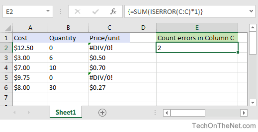
Let's show you how to count the number of errors in column C of a spreadsheet. Based on the spreadsheet below:
In cell E2, we've created the following array formula that uses the ISERROR function with the SUM function to count the number of errors in column C:
=SUM(ISERROR(C:C)*1)
When creating your array formula, you need to use Ctrl+Shift+Enter instead of Enter. This creates {} brackets around your formula as follows:
{=SUM(ISERROR(C:C)*1)}
This formula will check each value in column C for an error using the ISERROR function and return each error as a value of 1. The SUM function will then count those errors and return the total number of errors found in column C.
In this example, there are 2 errors in column C - the values found in cell C2 and C5 both contain the #DIV/0! error.
More Examples
Here are more examples that show how to use the ISERROR function in Excel:
Advertisements