

MS Excel: How to use the IFERROR Function (WS)
This Excel tutorial explains how to use the Excel IFERROR function with syntax and examples.
Description
The Microsoft Excel IFERROR function returns an alternate value if a formula results in an error. It will check for errors such as #N/A, #VALUE!, #REF!, #DIV/0!, #NUM!, #NAME? or #NULL.
The IFERROR function is a built-in function in Excel that is categorized as a Logical Function. It can be used as a worksheet function (WS) in Excel. As a worksheet function, the IFERROR function can be entered as part of a formula in a cell of a worksheet.
If you want to follow along with this tutorial, download the example spreadsheet.
Syntax
The syntax for the IFERROR function in Microsoft Excel is:
IFERROR( formula, alternate_value )
Parameters or Arguments
- formula
- The formula or value that you want to test.
- alternate_value
- The alternate value that is returned if the formula results in an error value (#N/A, #VALUE!, #REF!, #DIV/0!, #NUM!, #NAME? or #NULL). Otherwise, the function will return the result of the formula if no error occurs.
Returns
The IFERROR function returns any datatype such as a string, numeric, date, etc.
Applies To
- Excel for Office 365, Excel 2019, Excel 2016, Excel 2013, Excel 2011 for Mac, Excel 2010, Excel 2007
Type of Function
- Worksheet function (WS)
Example (as Worksheet Function)
Let's look at some Excel IFERROR function examples and explore how to use the IFERROR function as a worksheet function in Microsoft Excel:
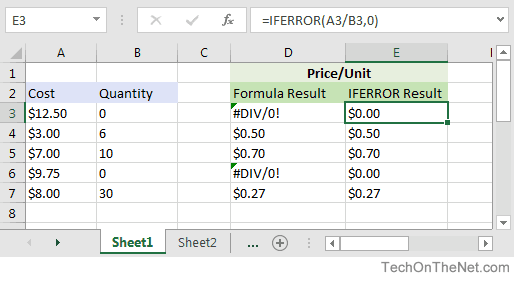
Based on the Excel spreadsheet above, column D contains the formula to calculate Price/Unit (for example, cell D3 contains the formula A3/B3). Because cells B3 and B6 contain 0 values, the formula results in #DIV/0! errors in cells D3 and D6.
Column E uses the IFERROR function to return an alternate value of 0 when the formula results in an error.
For example, the IFERROR function in cell E3 would return a value of 0 (ie: the alternate value) because A3/B3 results in the #DIV/0! error:
=IFERROR(A3/B3,0)
Result: 0
However, the IFERROR function in cell E4 would return $0.50:
=IFERROR(A4/B4,0)
Result: $0.50
Because A4/B4 does not result in an error, the function would return the result of the formula which is $0.50.
The IFERROR is an amazing function that can be used to trap and handle errors in your Excel formulas.
Advertisements