MS Excel: How to use the MODE.MULT Function (WS)

This Excel tutorial explains how to use the Excel MODE.MULT function with syntax and examples.

Description

The Microsoft Excel MODE.MULT function returns a vertical array of the most frequently occurring numbers found in a set of numbers. This function is useful if there is more than one number that occurs the most.

The MODE.MULT function is a built-in function in Excel that is categorized as a Statistical Function. It can be used as a worksheet function (WS) in Excel. As a worksheet function, the MODE.MULT function can be entered as part of a formula in a cell of a worksheet.

If you want to follow along with this tutorial, download the example spreadsheet.

Download Example

Syntax

The syntax for the MODE.MULT function in Microsoft Excel is:

MODE.MULT( number1, [number2, ... number_n] )

Parameters or Arguments

number1, number2, ... number_n

Each number can be a range, a cell or a numeric value. There can be up to 255 numbers.

Returns

The MODE.MULT function returns a vertical array of numeric values if entered as an array formula. It returns only a single numeric value if not entered as a regular formula.
If all numeric values in the set are unique, the MODE.MULT function returns the #N/A error.
If a text value such as "G" is entered as a parameter, the MODE.MULT function will return the #VALUE! error.
If a range or cell reference contains non-numeric values such as text values, logical values or empty cells, these values will be ignored.

Note

• See also MODE.SNGL and MODE functions.

Applies To

• Excel for Office 365, Excel 2019, Excel 2016, Excel 2013, Excel 2011 for Mac, Excel 2010

Type of Function

• Worksheet function (WS)

Example (as Worksheet Function)

Let's look at some Excel MODE.MULT function examples and explore how to use the MODE.MULT function as a worksheet function in Microsoft Excel:

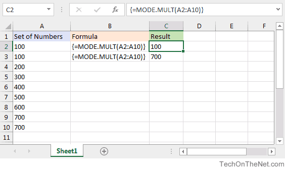
Based on the Excel spreadsheet above, the following MODE.MULT examples would return:

{=MODE.MULT(A2:A10)}
Result: 100    'First mode in vertical array (results in cell C2)

{=MODE.MULT(A2:A10)}
Result: 700    'Second mode in vertical array (results in cell C3)

How to Enter an Array Formula

The MODE.MULT function will return multiple modes if entered as an array formula, but how do you enter an array formula?

Let's show you how!

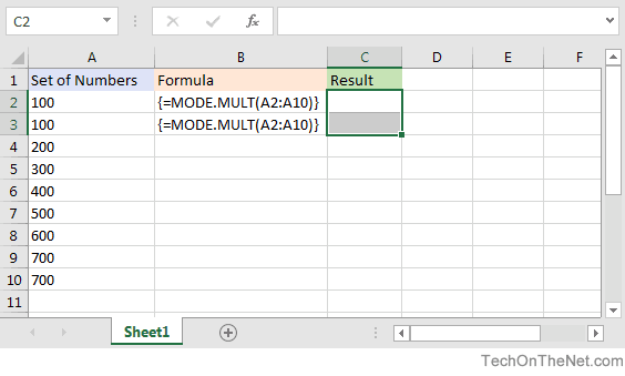
First, highlight the cells where you would like to display the results of the MODE.MULT function. In this example, we have highlighted cells C2:C3.

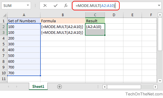
Next, type the MODE.MULT formula in the formula bar (but do not press the ENTER key). In this example, we have typed the formula:

=MODE.MULT(A2:A10)

Now, press Ctrl+Shift+Enter to create your formula as an array formula. This adds {} brackets around your formula as follows:

{=MODE.MULT(A2:A10)}

Now cells C2 and C3 will display the results of the MODE.MULT function as a vertical array with the first mode in cell C2 and the second mode in cell C3.

Since the array formula is tied to both cells C2 and C3, you must highlight the entire C2:C3 range to edit or clear the array formula.

{=TRANSPOSE(MODE.MULT(A2:A10))}