MS Excel: How to use the IFS function (WS)

This Excel tutorial explains how to use the Excel IFS function with syntax and examples.

Description

The Microsoft Excel IFS function lets you specify multiple IF conditions within one function call.

The IFS function is a built-in function in Excel that is categorized as a Logical Function. It can be used as a worksheet function (WS) in Excel. As a worksheet function, the IFS function can be entered as part of a formula in a cell of a worksheet.

This function replaces the old method of nesting multiple IF functions and lets you enter up to 127 conditions making your formulas easy to read and understand. The only downside to this function is that you can't specify an ELSE condition, but we do have a workaround which we will show you later in the tutorial.

Subscribe

---

If you want to follow along with this tutorial, download the example spreadsheet.

Download Example

Syntax

The syntax for the IFS function in Microsoft Excel is:

IFS( condition1, return1 [,condition2, return2] ... [,condition127, return127] )

Parameters or Arguments

condition1, condition2, ... condition127

The condition that you want to test. There can be up to 127 conditions entered.

return1, return2, ... return127

The value that is returned if the corresponding condition is TRUE. All conditions are evaluated in the order that they are listed so once the function finds a condition that evaluates to TRUE, the IFS function will return the corresponding value and stop processing any further conditions.

Returns

The IFS function returns any datatype such as a string, numeric, date, etc.
If none of the conditions evaluate to TRUE, the IFS function will return the #N/A error.

Applies To

• Excel for Office 365, Excel 2019

Type of Function

• Worksheet function (WS)

Example (as Worksheet Function)

Let's explore how to use the IFS function as a worksheet function in Microsoft Excel.

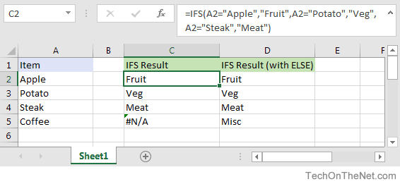
Based on the Excel spreadsheet above, the following IFS examples would return:

=IFS(A2="Apple","Fruit",A2="Potato","Veg",A2="Steak","Meat")
Result: "Fruit"

=IFS(A3="Apple","Fruit",A3="Potato","Veg",A3="Steak","Meat")
Result: "Veg"

=IFS(A4="Apple","Fruit",A4="Potato","Veg",A4="Steak","Meat")
Result: "Meat"

=IFS(A5="Apple","Fruit",A5="Potato","Veg",A5="Steak","Meat")
Result: #N/A

As you can see, we can enter multiple conditions in the IFS function. When a condition evaluates to TRUE, the corresponding value will be returned. However, if none of the conditions evaluate to TRUE, the #N/A error is returned which is shown in cell C5 in the example.

We can workaround this #N/A error by creating a "make-shift" ELSE condition. Let's explore this further.

Adding an ELSE Condition

To avoid getting a #N/A error, create one final condition at the end of the formula that is TRUE and then place the value that you would like returned as the ELSE condition.

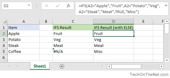
In this example, we have changed our formula from:

=IFS(A2="Apple","Fruit",A2="Potato","Veg",A2="Steak","Meat")

to

=IFS(A2="Apple","Fruit",A2="Potato","Veg",A2="Steak","Meat",TRUE,"Misc")

The addition of the final condition ,TRUE,"Misc" will allow us to return the value "Misc" when none of the previous conditions in the IFS function evaluate to TRUE.

The IFS function is a fantastic function and a great addition to Office 365 and Excel 2019. Give it a try!