MS Excel: How to use the MIRR Function (WS, VBA)

This Excel tutorial explains how to use the Excel MIRR function with syntax and examples.

Description

The Microsoft Excel MIRR function returns the modified internal rate of return for a series of cash flows. The internal rate of return is calculated by using both the cost of the investment and the interest received by reinvesting the cash.

The cash flows must occur at regular intervals, but do not have to be the same amounts for each interval.

The MIRR function is a built-in function in Excel that is categorized as a Financial Function. It can be used as a worksheet function (WS) and a VBA function (VBA) in Excel. As a worksheet function, the MIRR function can be entered as part of a formula in a cell of a worksheet. As a VBA function, you can use this function in macro code that is entered through the Microsoft Visual Basic Editor.

Syntax

The syntax for the MIRR function in Microsoft Excel is:

MIRR( range, finance_rate, reinvestment_rate )

Parameters or Arguments

range

A range of cells that represent the series of cash flows.

finance_rate

The interest rate that you pay on the cash flow amounts.

reinvestment_rate

The interest rate that you receive on the cash flow amounts as they are reinvested.

Returns

The MIRR function returns a numeric value.

Applies To

• Excel for Office 365, Excel 2019, Excel 2016, Excel 2013, Excel 2011 for Mac, Excel 2010, Excel 2007, Excel 2003, Excel XP, Excel 2000

Type of Function

• Worksheet function (WS)
• VBA function (VBA)

Example (as Worksheet Function)

Let's look at some Excel MIRR function examples and explore how to use the MIRR function as a worksheet function in Microsoft Excel:

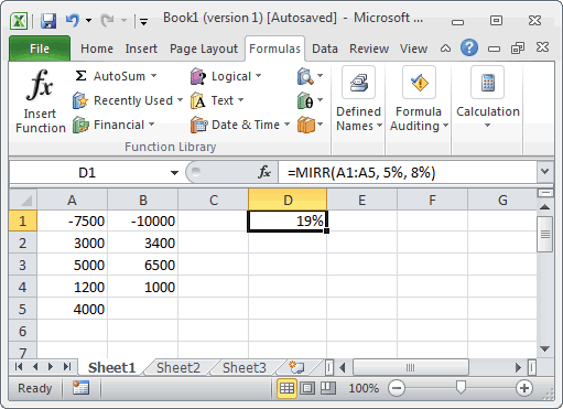
Based on the Excel spreadsheet above:

This first example returns a modified internal rate of return of 19%. It assumes that you start a business at a cost of $7,500 - this amount was borrowed at a rate of 5%. You net the following income for the first four years: $3,000, $5,000, $1,200, and $4,000. The net income was reinvested at a rate of 8%.

=MIRR(A1:A5, 5%, 8%)
Result: 19%

This next example returns a modified internal rate of return of 7%. It assumes that you start a business at a cost of $10,000 - this amount was borrowed at a rate of 6.5%. You net the following income for the first three years: $3,400, $6,500, and $1,000. The net income was reinvested at a rate of 10%.

=MIRR(B1:B4, 6.5%, 10%)
Result: 7%

Example (as VBA Function)

The MIRR function can also be used in VBA code in Microsoft Excel.

For example:

Dim LNumber As Double
Static Values(5) As Double

Values(0) = -7500
Values(1) = 3000
Values(2) = 5000
Values(3) = 1200
Values(4) = 4000

LNumber = Mirr(Values(), 0.05, 0.08)

In this example, the variable called LNumber would now contain the value of 0.16506818.