

MS Excel: How to use the HLOOKUP Function (WS)
This Excel tutorial explains how to use the Excel HLOOKUP function with syntax and examples. How to handle errors such as #N/A and retrieve the correct results is also discussed.
Description
The Microsoft Excel HLOOKUP function performs a horizontal lookup by searching for a value in the top row of the table and returning the value in the same column based on the index_number.
The HLOOKUP function is a built-in function in Excel that is categorized as a Lookup/Reference Function. It can be used as a worksheet function (WS) in Excel. As a worksheet function, the HLOOKUP function can be entered as part of a formula in a cell of a worksheet.
If you want to follow along with this tutorial, download the example spreadsheet.
Syntax
The syntax for the HLOOKUP function in Microsoft Excel is:
HLOOKUP( value, table, index_number, [approximate_match] )
Parameters or Arguments
- value
- The value to search for in the first row of the table.
- table
- Two or more rows of data that is sorted in ascending order.
- index_number
- The row number in table from which the matching value must be returned. The first row is 1.
- approximate_match
- Optional. Enter FALSE to find an exact match. Enter TRUE to find an approximate match. If this parameter is omitted, TRUE is the default.
Returns
The HLOOKUP function returns any datatype such as a string, numeric, date, etc.
If you enter FALSE for the approximate_match parameter and no exact match is found, then the HLOOKUP function will return #N/A.
If you specify TRUE for the approximate_match parameter and no exact match is found, then the next smaller value is returned.
If index_number is less than 1, the HLOOKUP function will return #VALUE!.
If index_number is greater than the number of columns in table, the HLOOKUP function will return #REF!.
Note
- See also the VLOOKUP function to perform a vertical lookup.
- See also the XLOOKUP function which is the next generation lookup function that works for both vertical and horizontal lookups.
Applies To
- Excel for Office 365, Excel 2019, Excel 2016, Excel 2013, Excel 2011 for Mac, Excel 2010, Excel 2007, Excel 2003, Excel XP, Excel 2000
Type of Function
- Worksheet function (WS)
Example (as Worksheet Function)
Let's explore how to use the HLOOKUP function as a worksheet function in Microsoft Excel:
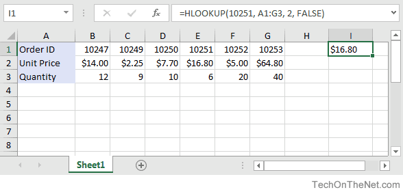
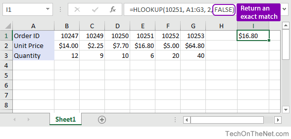
Based on the Excel spreadsheet above, the following HLOOKUP examples would return:
=HLOOKUP(10251, A1:G3, 2, FALSE)
Result: $16.80    'Returns value in 2nd row

=HLOOKUP(10251, A1:G3, 3, FALSE)
Result: 6         'Returns value in 3rd row

=HLOOKUP(10248, A1:G3, 2, FALSE)
Result: #N/A      'Returns #N/A error (no exact match)

=HLOOKUP(10248, A1:G3, 2, TRUE)
Result: $14.00    'Returns an approximate match
Now, let's look at the example =HLOOKUP(10251, A1:G3, 2, FALSE) that returns a value of $16.80 and take a closer look why.
First Parameter
The first parameter in the HLOOKUP function is the value to search for in the table of data.
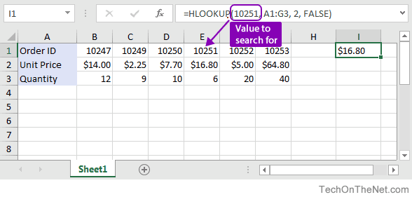
In this example, the first parameter is 10251. This is the value that the HLOOKUP will search for in the first row of the table of data.
Second Parameter
The second parameter in the HLOOKUP function is the table or source of data where the horizontal lookup should be performed.
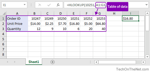
In this example, the second parameter is A1:G3. The HLOOKUP uses the first row in this range (ie: A1:G1) to search for the value of 10251.
Third Parameter
The third parameter is the position number in the table where the return data can be found. A value of 1 indicates the first row in the table. The second row is 2, and so on.
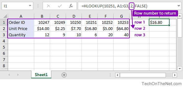
In this example, the third parameter is 2. This means that the second row in the table is where we will find the value to return. Since the table range is set to A1:G3, the return value will be in the second row somewhere in the range A2:G2.
Fourth Parameter
Finally and most importantly is the fourth or last parameter in the HLOOKUP. This parameter determines whether you are looking for an exact match or approximate match.
In this example, the fourth parameter is FALSE. A parameter of FALSE means that HLOOKUP is looking for an EXACT match for the value of 10251. A parameter of TRUE means that a "close" match will be returned. Since the HLOOKUP is able to find the value of 10251 in the range A1:G1, it returns the corresponding value from A2:G2 which is $16.80.
Exact Match vs. Approximate Match
To find an exact match, use FALSE as the final parameter. To find an approximate match, use TRUE as the final parameter.
Let's lookup a value that does not exist in our data to demonstrate the importance of this parameter!
Exact Match
Use FALSE to find an exact match:
=HLOOKUP(10248, A1:G3, 2, FALSE)
Result: #N/A
If no exact match is found, #N/A is returned.
Approximate Match
Use TRUE to find an approximate match:
=HLOOKUP(10248, A1:G3, 2, TRUE)
  Result: $14.00
If no match is found, it returns the next smaller value which in this case is $14.00.
HLOOKUP from Another Sheet
You can use the HLOOKUP to lookup a value when the table is on another sheet. Let's modify our example above and assume that the table is in a different Sheet called Sheet2 in the range A1:G3. We could rewrite our original example where we lookup the value 10251 as follows:
=HLOOKUP(10251, Sheet2!A1:G3, 2, FALSE)
By preceding the table range with the sheet name and an exclamation mark, we can update our HLOOKUP to reference a table on another sheet.
HLOOKUP from Another Sheet with Spaces in Sheet Name
Let's throw in one more complication. What happens if your sheet name contains spaces? If there are spaces in the sheet name, you will need to change the formula further.
Let's assume that the table is on a Sheet called "Test Sheet" in the range A1:G3, we would need to modify our formula as follows:
=HLOOKUP(10251, 'Test Sheet'!A1:G3, 2, FALSE)
By placing the sheet name within single quotes, we can accommodate a sheet name with spaces in our HLOOKUP function.
Why use Absolute Referencing?
Now it is important for us to mention one more mistake that is commonly made. When people use the HLOOKUP function, they commonly use relative referencing for the table range like we did in our examples above. This will return the right answer, but what happens when you copy the formula to another cell? The table range will be adjusted by Excel and change relative to where you paste the new formula. Let's explain further...
So if you had the following formula in cell J1:
=HLOOKUP(10251, A1:G3, 2, FALSE)
And then you copied this formula from cell J1 to cell K2, it would modify the HLOOKUP formula to this:
=HLOOKUP(10251, B2:H4, 2, FALSE)
Since your table is found in the range A1:G3 and not B2:H4, your formula would return erroneous results in cell K2. To ensure that your range is not changed, try referencing your table range using absolute referencing as follows:
=HLOOKUP(10251, $A$1:$G$3, 2, FALSE)
Now if you copy this formula to another cell, your table range will remain $A$1:$G$3.
How to Handle #N/A Errors
Finally, let's look at how to handle instances where the HLOOKUP function does not find a match and returns the #N/A error. In most cases, you don't want to see #N/A but would rather display a more user-friendly result.
For example, if you had the following formula:
=HLOOKUP(10248, $A$1:$G$3, 2, FALSE)
Instead of displaying #N/A error if you do not find a match, you could return the value "Not Found". To do this, you could modify your HLOOKUP formula as follows:
=IF(ISNA(HLOOKUP(10248, $A$1:$G$3, 2, FALSE)), "Not Found", HLOOKUP(10251, $A$1:$F$2, 2, FALSE))
OR
=IFERROR(HLOOKUP(10248, $A$1:$G$3, 2, FALSE), "Not Found")
OR
=IFNA(HLOOKUP(10248, $A$1:$G$3, 2, FALSE), "Not Found")
These formulas use the ISNA, IFERROR and IFNA functions to return "Not Found" if a match is not found by the HLOOKUP function.
This is a great way to spruce up your spreadsheet so that you don't see traditional Excel errors.
Advertisements