MS Excel: How to use the FIND Function (WS)

This Excel tutorial explains how to use the Excel FIND function with syntax and examples.

Description

The Microsoft Excel FIND function returns the location of a substring in a string. The search is case-sensitive.

The FIND function is a built-in function in Excel that is categorized as a String/Text Function. It can be used as a worksheet function (WS) in Excel. As a worksheet function, the FIND function can be entered as part of a formula in a cell of a worksheet.

Subscribe

---

If you want to follow along with this tutorial, download the example spreadsheet.

Download Example

Syntax

The syntax for the FIND function in Microsoft Excel is:

FIND( substring, string, [start_position] )

Parameters or Arguments

substring

The substring that you want to find.

string

The string to search within.

start_position

Optional. It is the position in string where the search will start. The first position is 1. If the start_position is not provided, the FIND function will start the search at the beginning of the string.

Returns

The FIND function returns a numeric value. The first position in the string is 1.
If the FIND function does not find a match, it will return a #VALUE! error.

Applies To

• Excel for Office 365, Excel 2019, Excel 2016, Excel 2013, Excel 2011 for Mac, Excel 2010, Excel 2007, Excel 2003, Excel XP, Excel 2000

Type of Function

• Worksheet function (WS)

Example (as Worksheet Function)

Let's look at some Excel FIND function examples and explore how to use the FIND function as a worksheet function in Microsoft Excel:

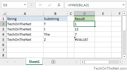
Based on the Excel spreadsheet above, the following FIND examples would return:

=FIND(B2,A2)
Result: 1

=FIND("T",A2)
Result: 1

=FIND("t",A3)
Result: 12

=FIND("The",A4)
Result: 7

=FIND("Z",A5)
Result: #VALUE!

=FIND("T", A2, 3)
Result: 7

Frequently Asked Questions

Question: In Microsoft Excel, I have the value "Supermarket" in cell A1 and 100 in cell A2.

Objective: If A1 contains "Super", then I want A3=A2. Otherwise, I want A3=0. I'm unable to use the FIND function because if cell A1 does not contain "Super", the FIND function returns the #VALUE! error which does not let me sum column A.

Answer: To make sure that do not return any #VALUE! errors when using the FIND function, you need to also use the ISERROR function in your formula.

Let's look at an example.

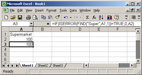
Based on the Excel spreadsheet above, the following FIND examples would return:

=IF(ISERROR(FIND("Super",A1,1))=TRUE,0,A2)
Result: 100

In this case, cell A1 does contain the value "Super", so the formula returns the value found in cell A2 which is 100.

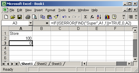
Based on the Excel spreadsheet above, the following FIND examples would return:

=IF(ISERROR(FIND("Super",A1,1))=TRUE,0,A2)
Result: 0

In this example, cell A1 does NOT contain the value "Super", so the formula returns 0.

Let's just quickly explain how this formula works. If cell A1 contains "Super", the FIND function will return the numerical position of the value of "Super". Thus, an error will not result (ie. the IsError function evaluates to FALSE) and the formula will return A2.

If cell A1 does NOT contain "Super", the FIND function will return the #VALUE! error causing the IsError function to evaluate to TRUE and return 0.