

MS Excel: Frequently Asked Questions for INDEX Function
Interested in learning more about the INDEX function? Here are some questions that others have asked about the INDEX function.
Frequently Asked Questions
Question:I have a question about how to nest a MATCH function within the INDEX function. The question is:
I want to create a formula using the MATCH function nested within the INDEX function to retrieve the Class that was selected (by the x) in E4:F10. The MATCH function should find the row where the x is located and should be used within the INDEX function to retrieve the associated Class value from the same row within F4:F10.
Answer:We can use the MATCH function to find the row position in the range E4:E10 to find the row where "x" is located. We then embed this MATCH function within the INDEX function to return the corresponding value in the range F4:$10 as follow:
=INDEX($F$4:$F$10, MATCH("x",$E$4:$E$10), 1)
In this example, we are searching for the value "x" within the range E4:E10. When the value of "x" is found, it will return the corresponding value from F4:F10.
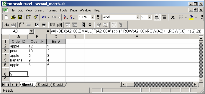
Question: Is there a simple way in Excel to VLOOKUP the second match in a column? So, for instance, If I had apple, pear, apple listed in the column (each word in a separate cell), would there be a way to look up the values to the right of the second "apple"?
Answer: This can be done with a formula that utilizes a combination of the INDEX, SMALL and ROW functions.
If you wanted to return the quantity value for the second occurrence of apple, you would use the following array formula:
=INDEX(A2:C6,SMALL(IF(A2:C6="apple",ROW(A2:C6)-ROW(A2)+1,ROW(C6)+1),2),2)
When creating your array formula, you need to use Ctrl+Shift+Enter instead of Enter. This creates {} brackets around your formula as follows:
{=INDEX(A2:C6,SMALL(IF(A2:C6="apple",ROW(A2:C6)-ROW(A2)+1,ROW(C6)+1),2),2)}
If you wanted to return the quantity value for the third occurrence of apple, you would use the following array formula:
=INDEX(A2:C6,SMALL(IF(A2:C6="apple",ROW(A2:C6)-ROW(A2)+1,ROW(C6)+1),3),2)
When creating your array formula, you need to use Ctrl+Shift+Enter instead of Enter. This creates {} brackets around your formula as follows:
{=INDEX(A2:C6,SMALL(IF(A2:C6="apple",ROW(A2:C6)-ROW(A2)+1,ROW(C6)+1),3),2)}
If you wanted to return the bin # for the second occurrence of apple, you would use the following array formula:
=INDEX(A2:C6,SMALL(IF(A2:C6="apple",ROW(A2:C6)-ROW(A2)+1,ROW(C6)+1),2),3)
When creating your array formula, you need to use Ctrl+Shift+Enter instead of Enter. This creates {} brackets around your formula as follows:
{=INDEX(A2:C6,SMALL(IF(A2:C6="apple",ROW(A2:C6)-ROW(A2)+1,ROW(C6)+1),2),3)}
Advertisements