

MS Excel 2003: How to Show Bottom 10 Results in a Pivot Table
This Excel tutorial explains how to show the bottom 10 results in a pivot table in Excel 2003 and older versions (with screenshots and step-by-step instructions).
See solution in other versions of Excel:
Question: How do I show only the bottom 10 results in a pivot table in Microsoft Excel 2003/XP/2000/97?
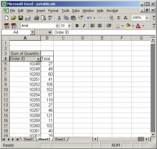
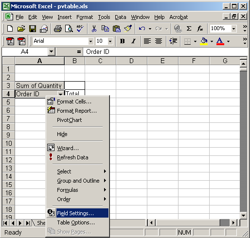
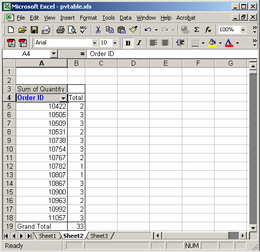
Answer: Select the row heading in the pivot table. In this example, we are selecting the Order ID heading.
Right-click and then select "Field Settings" from the popup menu.
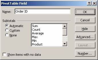
When the PivotTable Field window appears, click on the Advanced button.
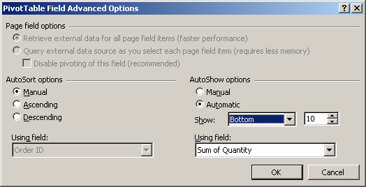
Under the AutoShow options, select Automatic. Select Bottom and the number of items that you wish to view. Now click on the OK button.
In this example, we've chosen the Bottom 10 values based on the "Sum of Quantity" field.
This will return you to the PivotTable Field window. Click on the OK button.
Now when you view your spreadsheet, you should only see the bottom 10 values based on quantity.


Advertisements