ADVERTISEMENT

MS Excel: Show Bottom 10 results in a pivot table in Excel 2011 for Mac

---

Question:  How do I show only the bottom 10 results in a pivot table in Excel 2011 for Mac?

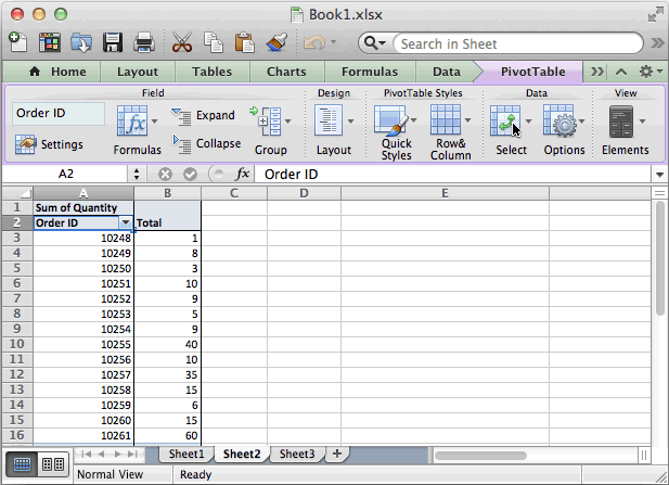
Answer:  In this example, we want to see the bottom 10 Order IDs based on the "Sum of Quantity".

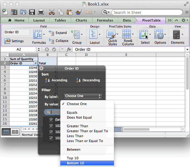
Click on the arrow to the right of the Order ID drop down box.

A popup window will appear. In this window, click on By value and select Bottom 10 from the popup menu.

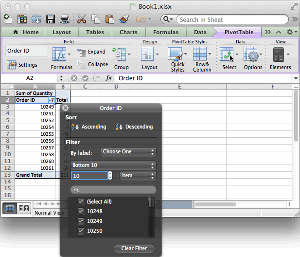
"Bottom 10" should appear in the window, replacing the "By value" drop down. Next, enter 10 in the field directly below to specify that you wish to see the bottom 10 items.

Then close this popup by clicking on the X in the top left of the popup.

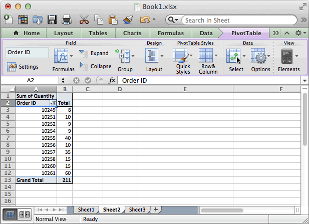
Now when you view your spreadsheet, you should only see the bottom 10 Order IDs based on the Sum of Quantity.