---

MS Excel 2003: How to Create a Pivot Table

This Excel tutorial explains how to create a pivot table in Excel 2003 and older versions (with screenshots and step-by-step instructions).

Question: How do I create a pivot table in Microsoft Excel 2003/XP/2000/97?

Answer: We'll start by creating a very simple pivot table. The example that follows has been done in Excel 2000, so the screen may look different if you are using a different version of Excel. Either way, it will give you a basic understanding of pivot tables.

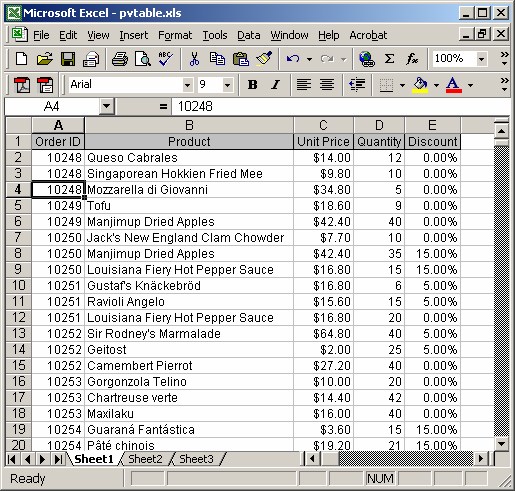
First, our data that we want to use to populate the pivot table resides on Sheet1.

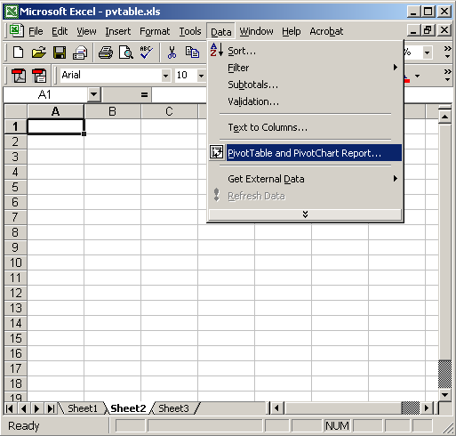
Under the Data menu, select "PivotTable and PivotChart Report".

A PivotTable wizard should appear. Make sure that the "Microsoft Excel list or database" and "PivotTable" options are chosen. Click on the Next button.

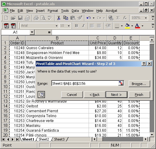
Select the range of data for the pivot table and click on the Next button. In this example, we've chosen data from Sheet1.

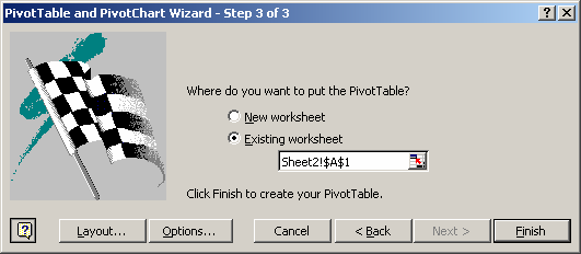
Select the position to create the new pivot table. It will automatically default to the cell that was highlighted when you started this process. In this example, we want to create our pivot table on Sheet2 in cell A1.

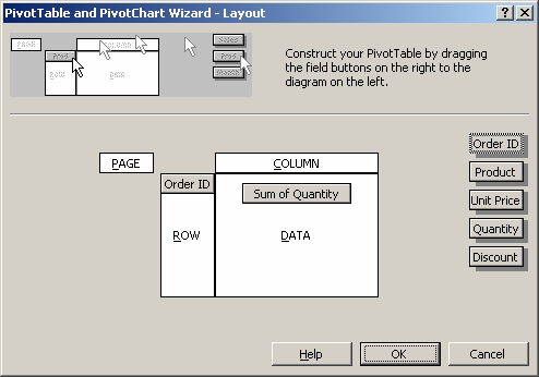
Click on the Layout button.

Now drag the fields that you want to appear in the Page, Row, Column, and Data sections of the pivot table. In this example, we've dragged the Order ID field to the Row section and the Quantity to the Data section.

Click on the OK button to continue.

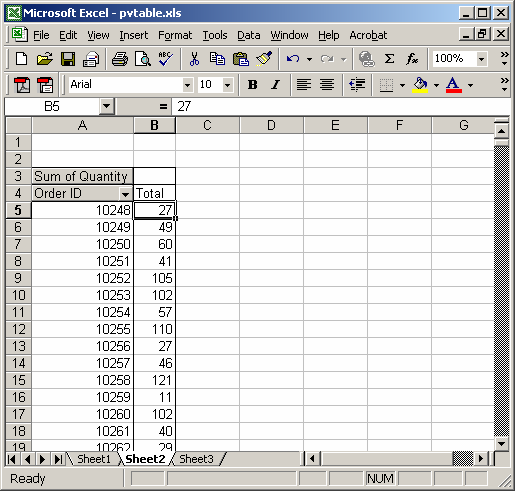
Now click on the Finish button.

Your pivot table should now appear on Sheet2. What this pivot table displays is the total quantity for each order ID.