

MS Excel 2016: How to Hide a Value in a Pivot Table
This Excel tutorial explains how to hide a value in a pivot table in Excel 2016 (with screenshots and step-by-step instructions).
See solution in other versions of Excel:
If you want to follow along with this tutorial, download the example spreadsheet.
Steps to Hide a Value in a Pivot Table
To hide a value in pivot table in Excel 2016, you will need to do the following steps:
-
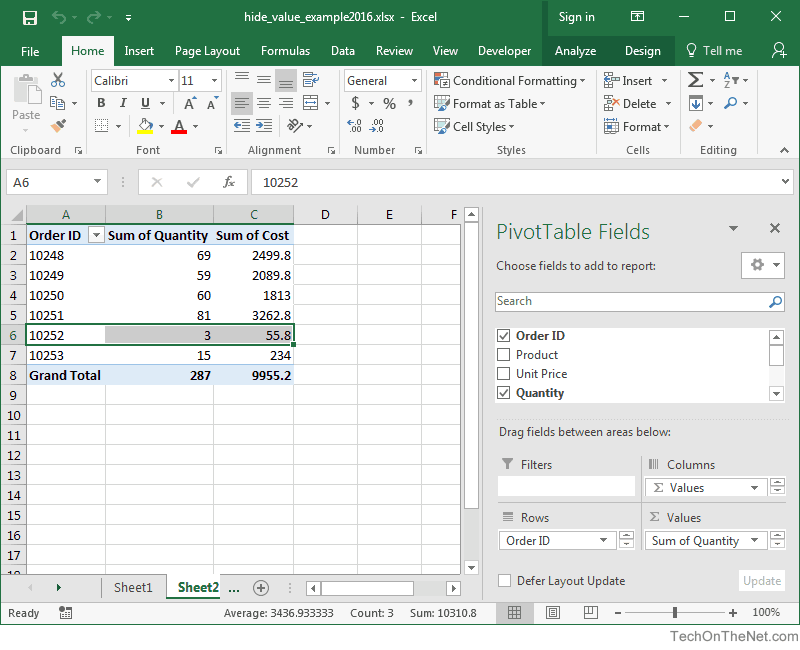
First, identify the value in the pivot table that you wish to hide. In this example, we are going to hide Order #10252.
-
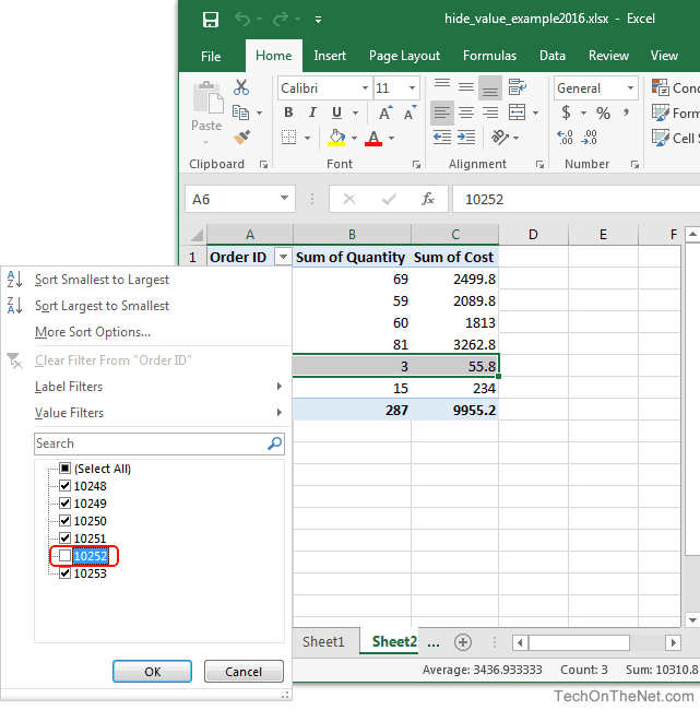
Click on the arrow to the right of the Order ID drop down box and un-select the checkbox next to the 10252 value. Then click on the OK button.
-
When you view the pivot table, Order #10252 is now hidden.
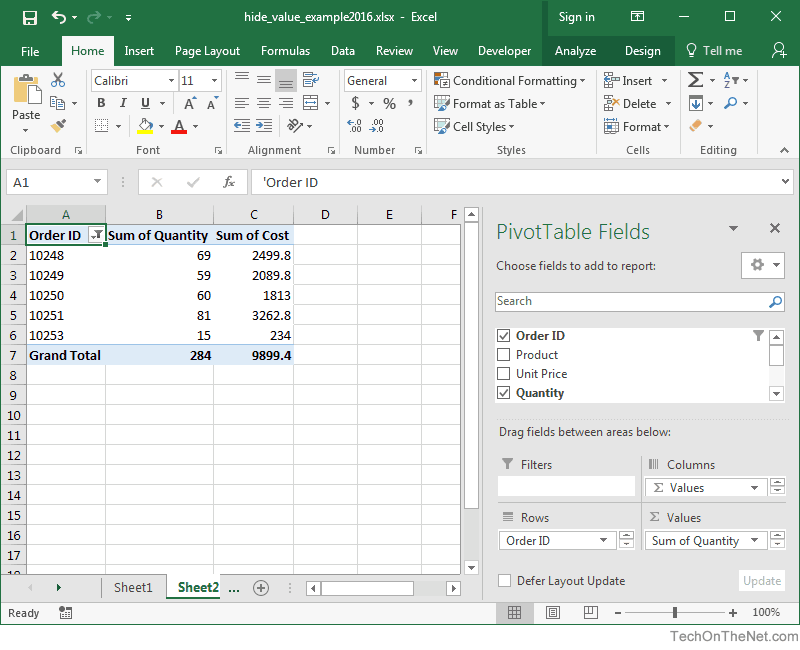 TIP: You will see the filter icon
 appear next to the Order ID heading when the value has been hidden.


Advertisements