

MS Excel 2016: How to Display a Hidden Value in a Pivot Table
This Excel tutorial explains how to unhide a value in a pivot table in Excel 2016 (with screenshots and step-by-step instructions).
See solution in other versions of Excel:
If you want to follow along with this tutorial, download the example spreadsheet.
Steps to Unhide a Value in a Pivot Table
To show a hidden value in pivot table in Excel 2016, you will need to do the following steps:
-
Look for the filter icon
 next to a pivot table heading. This indicates that a value has been hidden in the pivot table. In this example, Order #10252 has been hidden in the pivot table. We will show you how to unhide this value.
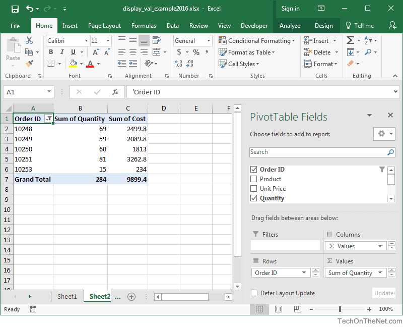
-
Click on the arrow to the right of the Order ID drop down box and select the checkbox for the 10252 value. Then click on the OK button.
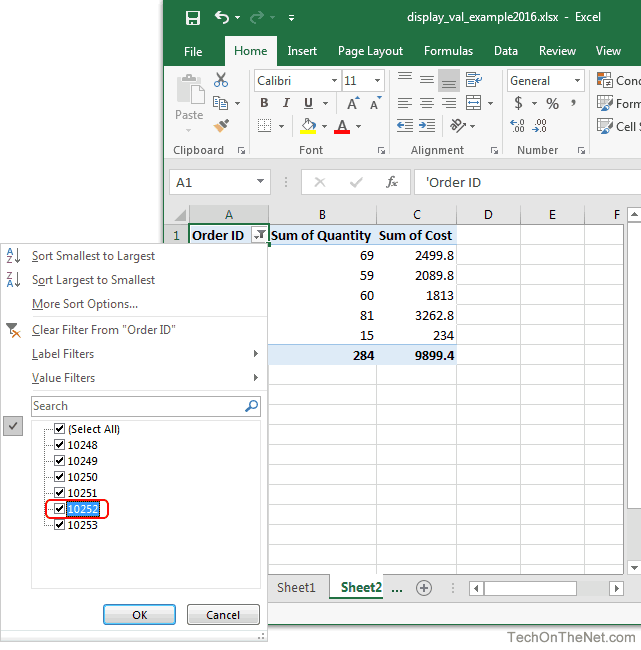 TIP: All checked values are visible in the pivot table. All unchecked values are hidden in the pivot table.
 -
Now we can see the details for Order ID 10252 in the pivot table and the filter icon
is no longer next to the Order ID heading.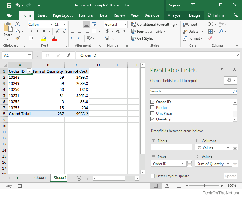


Advertisements