

MS Excel 2016: How to Handle Errors in a Pivot Table
This Excel tutorial explains how to change the display of errors in a pivot table in Excel 2013 (with screenshots and step-by-step instructions).
See solution in other versions of Excel:
If you want to follow along with this tutorial, download the example spreadsheet.
Steps to Handle Errors in a Pivot Table
When you have errors in a pivot table, you can replace the errors with an alternate value. Let's explore how to do this.
To replace pivot table errors in Excel 2016, you will need to do the following steps:
-
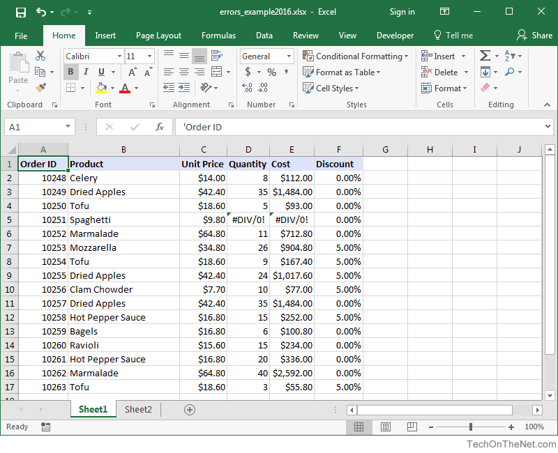
First, identify the errors in the source data for the pivot table. This will help you determine what value to use as the replacement for the error.
In this example, you can see #DIV/0! error in row 5 for both Quantity and Cost. This could be the result of a mathematical formula, for example.
-
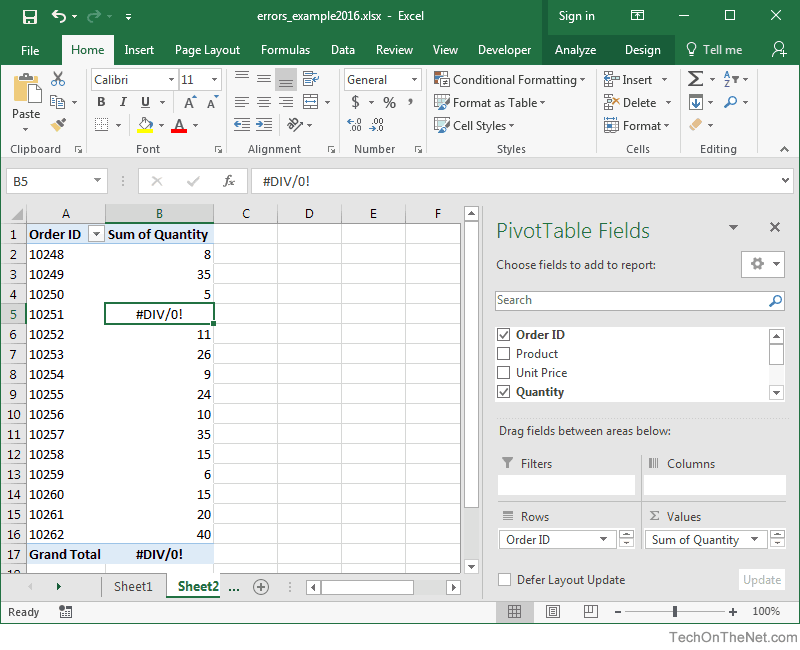
Now, select Sheet2 in the spreadsheet to see how the error appears in the pivot table.
-
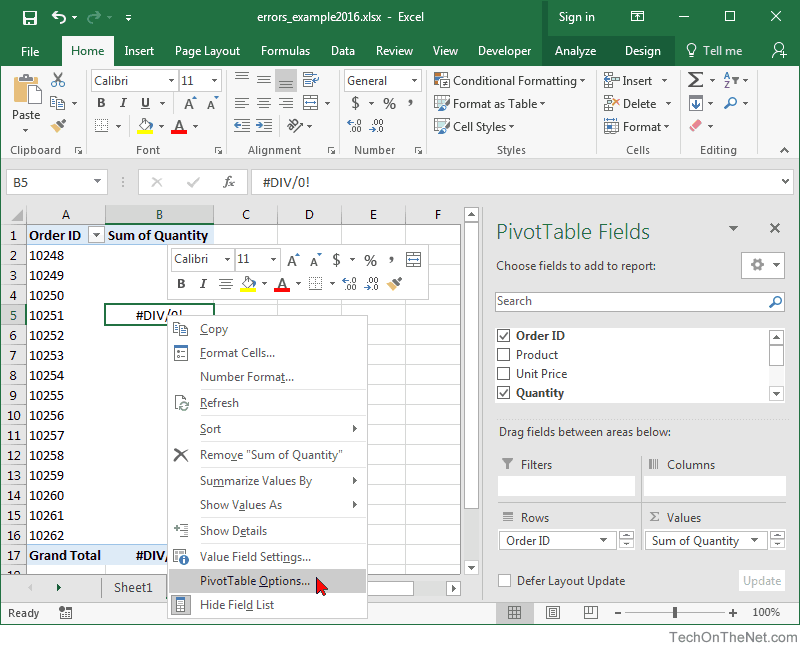
You can replace this error with a more appropriate value. To do this, right-click on the pivot table and then select PivotTable Options from the popup menu.
-
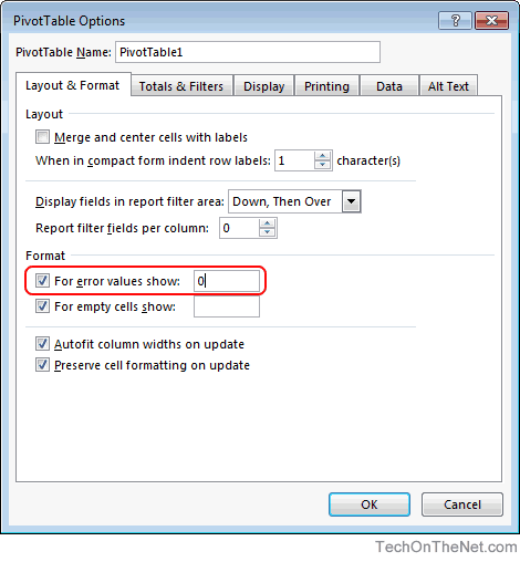
When the PivotTable Options window appears, check the checkbox called "For error values show". Then enter the value that you wish to see in the pivot table instead of the error. Click on the OK button. In this example, we've entered 0 so all errors in the pivot table will be replaced with the value of 0.
-
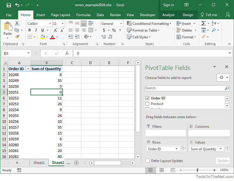
Now when we return to the pivot table, this is what we'll see. The error value has now been replaced with the value of 0.


Advertisements