---

MS Excel 2016: How to Change Data Source for a Pivot Table

This Excel tutorial explains how to change the data source for a pivot table in Excel 2016 (with screenshots and step-by-step instructions).

If you want to follow along with this tutorial, download the example spreadsheet.

Download Example

Steps to Change the Data Source of a Pivot Table

To change the data source of an existing pivot table in Excel 2016, you will need to do the following steps:

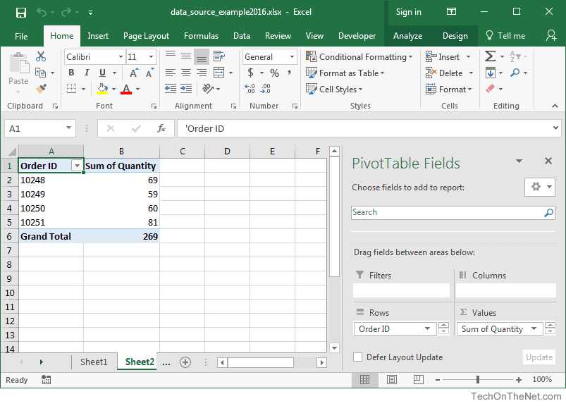
1. Select any cell in the pivot table to reveal more pivot table options in the toolbar. In this example, we have selected cell A1 on Sheet2.

   You now should see 2 new tabs appear in the toolbar called Analyze and Design.

   

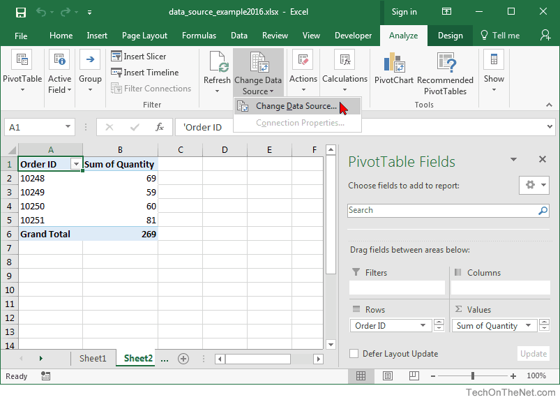
2. Select the Analyze tab from the toolbar at the top of the screen. In the Data group, click on Change Data Source button and select "Change Data Source" from the popup menu.

   

3. When the Change PivotTable Data Source window appears, change the Table/Range value to the new data source that you want for your pivot table and then click on the OK button.

   

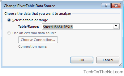
   In this example, we want to change the range from Sheet1!$A$1:$F$16 to Sheet1!$A$1:$F$17 because we have added one more row to our data in Sheet1.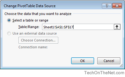

   

4. Now when you return to your pivot table, it should automatically refresh the pivot table and display the information from the new data source.

   

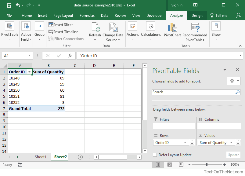
   In this example, Order ID 10252 now shows in the pivot table results.