

MS Excel 2016: Change how Empty Cells are Displayed in a Pivot Table
This Excel tutorial explains how to change the display of empty cells in a pivot table in Excel 2016 (with screenshots and step-by-step instructions).
See solution in other versions of Excel:
If you want to follow along with this tutorial, download the example spreadsheet.
Steps to Handle Empty Cells in a Pivot Table
When you have empty cells in a pivot table, you can replace the empty cells with an alternate value. Let's explore how to do this.
To replace empty cells in pivot table in Excel 2016, you will need to do the following steps:
-
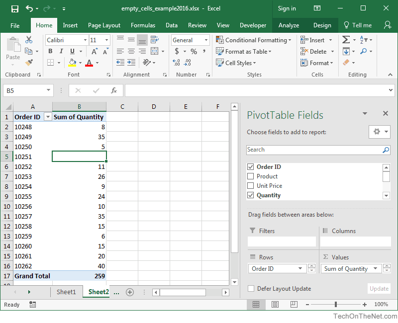
First, identify the empty cells in the pivot table. This will help you determine what value to use as the replacement for the empty cell.
In the example below, we have order #10251 that does not have a quantity value (row 5 in spreadsheet). Therefore, the quantity is showing as a blank or empty cell.
-
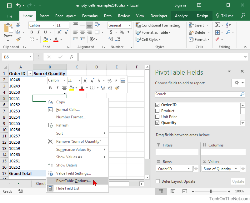
We'd like to replace all empty cells with the value "n/a". To do this, right-click on the pivot table and then select PivotTable Options from the popup menu.
-
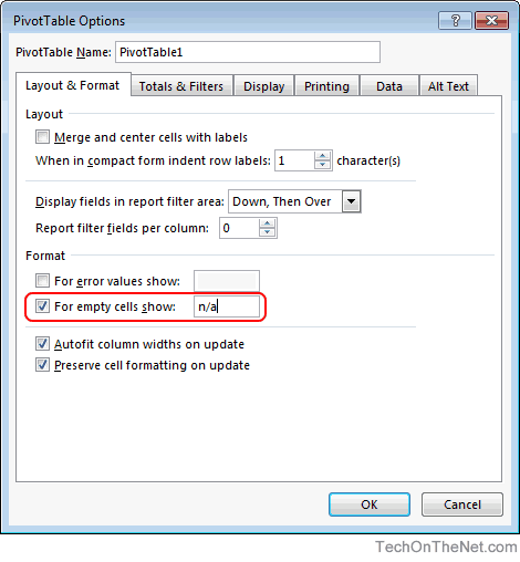
When the PivotTable window appears, check the checkbox called "For empty cells show". Then enter the value that you wish to see in the pivot table instead of the empty cell. Click on the OK button. In this example, we want all blank cells to show as "n/a".
-
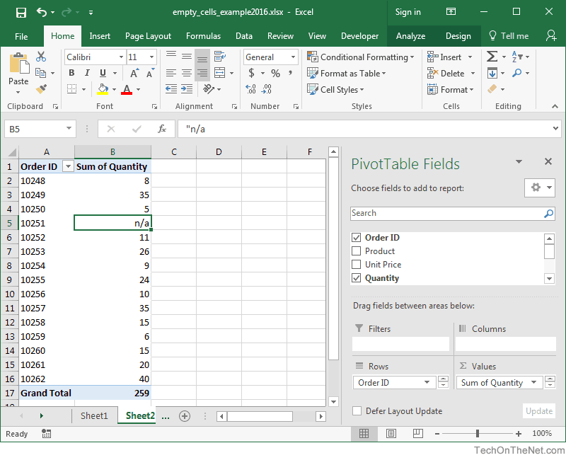
Now when we return to the pivot table, we see "n/a" as the Sum of Quantity value for order #10251.


Advertisements