

MS Excel 2016: How to Create a Pie Chart
This Excel tutorial explains how to create a basic pie chart in Excel 2016 (with screenshots and step-by-step instructions).
What is a Pie Chart?
A pie chart is a circle that is divided into slices and each slice represents a proportion of the whole.
It is a graphical object used to represent the data in your Excel spreadsheet that uses 1 series of data to create the graph.
You can use a pie chart when:
- You want to show numbers as a proportion of the whole (ie: the numbers equal 100%).
- There are a limited number of pie slices. If there are too many pie slices, then a pie chart is not a recommended graph to use.

If you want to follow along with this tutorial, download the example spreadsheet.
Steps to Create a Pie Chart
To create a pie chart in Excel 2016, you will need to do the following steps:
-
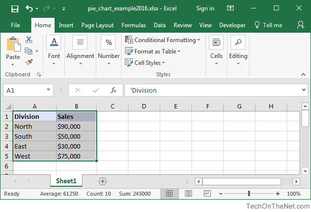
Highlight the data that you would like to use for the pie chart. In this example, we have selected the range A1:B5.
-
Select the Insert tab in the toolbar at the top of the screen. Click on the Pie Chart button
 in the Charts group and then select a chart from the drop down menu. In this example, we have selected the first pie chart (called Pie) in the 2-D Pie section.TIP: As you hover over each choice in the drop down menu, it will show you a preview of your data in the highlighted chart format.
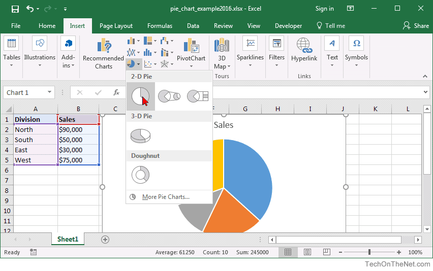
-
Now you will see the completed pie chart. In this tutorial, the pie chart has 4 slices (one for each division). Each slice represents the sales as a percentage of the total sales.
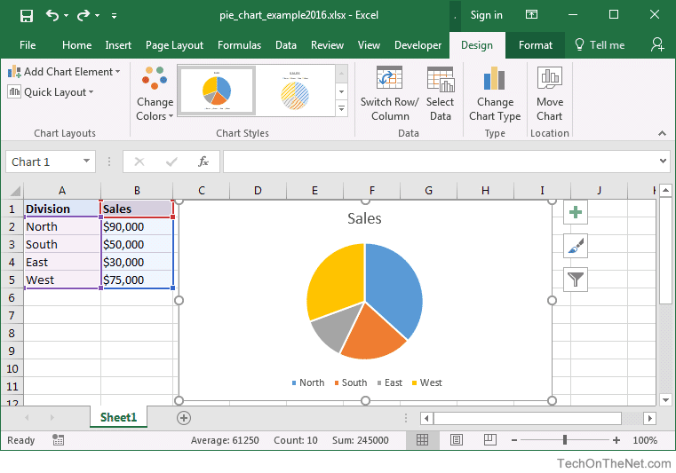
Congratulations, you have finished creating your first pie chart in Excel 2016!
Advertisements