---

MS Excel 2003: Exclude rows from the pivot table based on summed totals

This Excel tutorial explains how to exclude rows from the pivot table based on summed totals in Excel 2003 and older versions (with screenshots and step-by-step instructions).

Question: In Microsoft Excel 2003/XP/2000/97, I have a pivot table with sums that are in some cases zero. Note, that the values making them up are not zero (i.e. the values may be -1 and +1 producing a total of zero).

How can I exclude these rows from my pivot table? I don't believe hiding them is an option for reasons I can explain if you need me to.

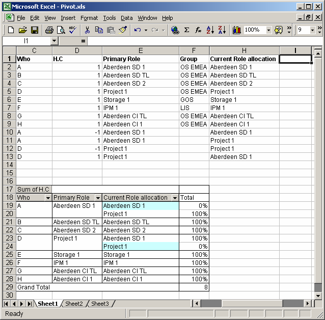
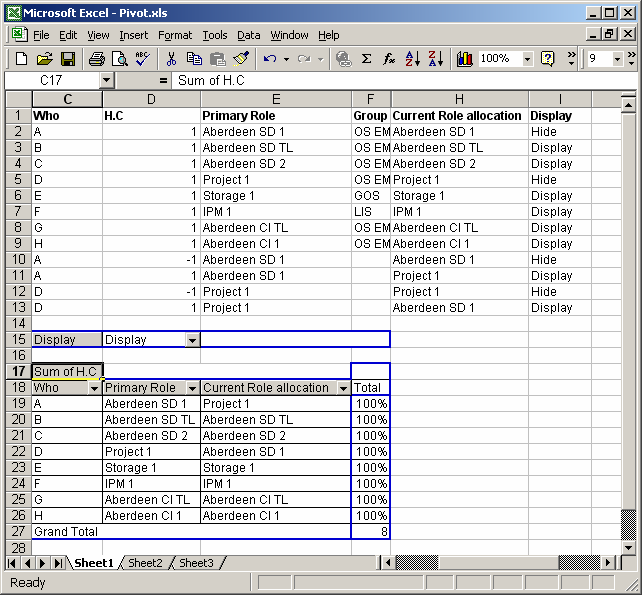
Answer: Let's look at an example. Below we have a pivot table that is based on the data in cells C1:H13. We want to exclude from the pivot tables the rows that are in blue in the pivot table. These are the rows whose Total sums to zero.

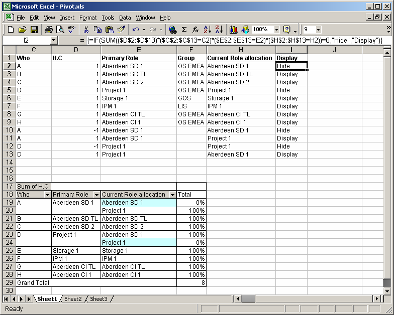
To do this, we'll need to add an extra column (column I) to the data which contains a label of "Hide" or "Display". We'll calculate this value based on an array formula that sums all HC values for the Who, Primary Role, and Current Role allocation combinations. If the sum adds up to zero, then the formula will return "Hide". Otherwise, it will return "Display".

In cell I2, e've created the following array formula:

=IF(SUM(($D$2:$D$13)*($C$2:$C$13=C2)*($E$2:$E$13=E2)*($H$2:$H$13=H2))=0,"Hide","Display")

When creating your array formula, you need to use Ctrl+Shift+Enter instead of Enter. This creates {} brackets around your formula as follows:

{=IF(SUM(($D$2:$D$13)*($C$2:$C$13=C2)*($E$2:$E$13=E2)*($H$2:$H$13=H2))=0,"Hide","Display")}

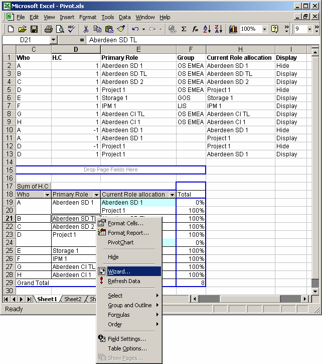
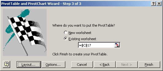
Now, we need to update our pivot table to include this new column. To do this, right-click on the pivot table and select Wizard from the popup menu.

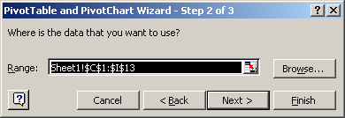
When the Wizard window appears, click on the Back button.

Then set the range to include the data in column I. So in this example, we set the range to:

Sheet1!$C$1:$I$13

Click on the Next button.

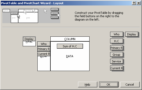
Then click on the Layout button.

When the Layout window appears, click on the Display field (in the field listing) and drag it to the Page section of the pivot table. Then click on the OK button.

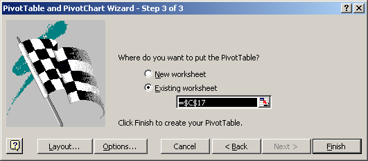
Then click on the Finish button.

Now when you return to your spreadsheet, you should see a Display field at the top of the pivot table.

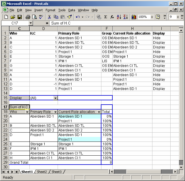
Click on the Display drop-down and select Display as the filter. Now, the zero Total values should disappear.