

MS Excel 2013: How to Change the Name of a Pivot Table
This Excel tutorial explains how to change the name of a pivot table in Excel 2013 (with screenshots and step-by-step instructions).
See solution in other versions of Excel:
If you want to follow along with this tutorial, download the example spreadsheet.
Steps to Change a Pivot Table Name
When you create a pivot table in Excel, there is a name associated with the pivot table. By default, the first pivot table you create is called PivotTable1, the second is PivotTable2, the third is PivotTable3, and so on. You can rename the pivot table to something more meaningful if you like. We recommend doing this if you plan to reference the pivot table in VBA code later.
To change the name of a pivot table in Excel 2013, you will need to do the following steps:
-
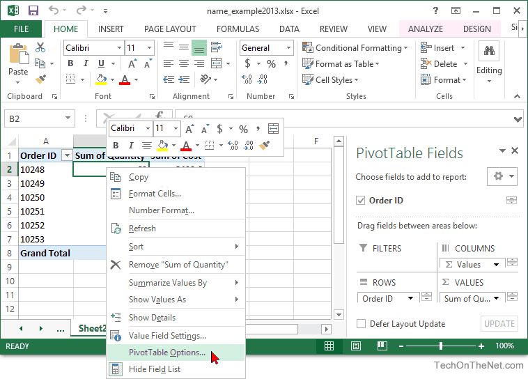
Right-click on the pivot table and then select "PivotTable Options" from the popup menu.
-
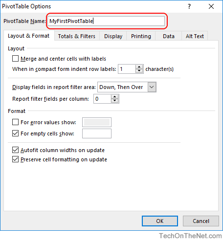
When the PivotTable Options window appears, enter the new name for the pivot table in the PivotTable Name field. Click the OK button. In this example, we've renamed our pivot table to MyFirstPivotTable.


Advertisements