---

MS Excel 2011 for Mac: Automatically highlight highest and lowest values in a range of cells

This Excel tutorial explains how to use conditional formatting to automatically highlight the highest and lowest values in a range of cells in Excel 2011 for Mac (with screenshots and step-by-step instructions).

Question: In Microsoft Excel 2011 for Mac, is there a way to shade one cell green if it is the highest value in a range of cells, and to shade another cell red if it is the lowest number in a range of cells?

Answer: Yes, you can use conditional formatting to highlight the highest and lowest values in a range of cells.

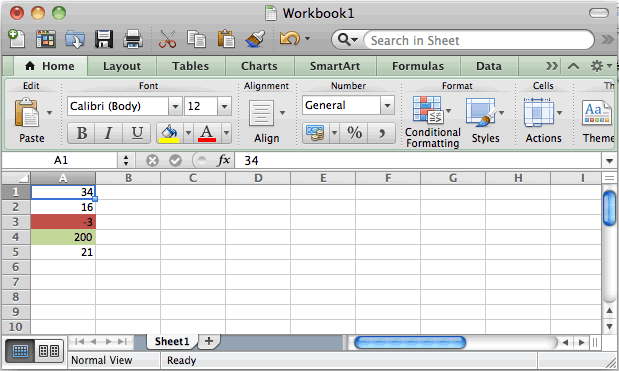
First highlight the range of cells. In this example, we've selected cells A1 through A5.

Select the Home tab in the toolbar at the top of the screen. Then click on the Conditional Formatting drop-down and select Manage Rules from the popup menu.

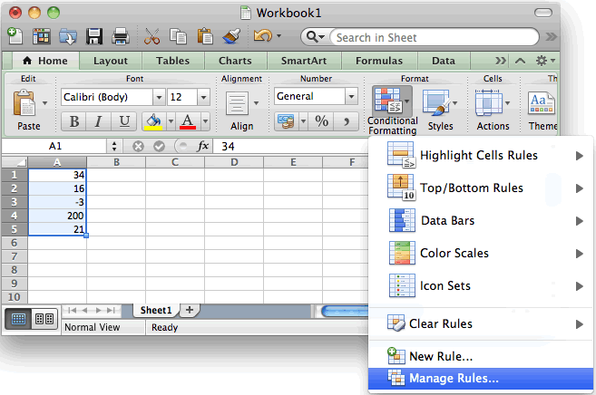
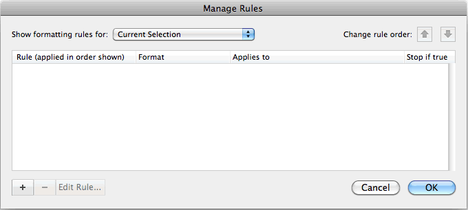
When the Manage Rules window appears, click on the + button in the bottom left to enter the first condition.

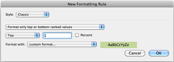
When the New Formatting Rule window appears, select Classic as the Style.

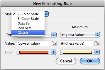
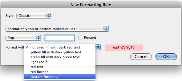
Then select Format only top or bottom ranked values in the first drop down, Top in the second drop down and enter 1 in the final box. In our example, we've selected only the first top value.

Next, we need to select what formatting to apply when this condition is met. To do this, select custom format from the Format with drop down.

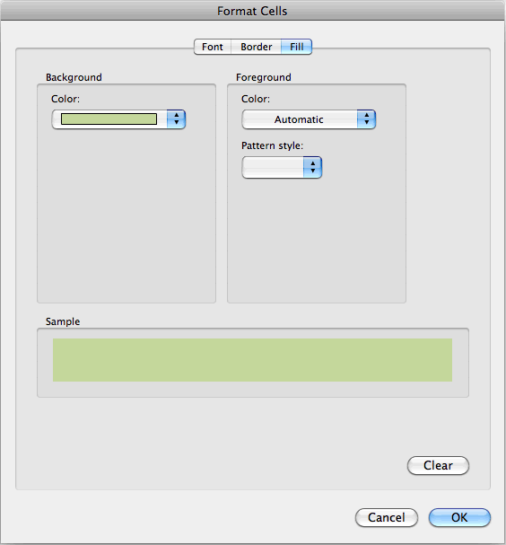
When the Format Cells window appears, select the Fill tab. Then select the color that you'd like to see for the highest value in the range. In this example, we've selected green. We also went to the Font tab and set the Color to Automatic.

Then click on the OK button.

When you return to the New Formatting Rule window, you should see the preview of the formatting in the Preview box. In this example, the preview box shows green as the fill color. Next click on the OK button.

This will return you to the Manage Rules window.

You will need to click on the + button again in the bottom left.

When the New Formatting Rule window appears, we need to set up the second condition.

Select Class as the Style.

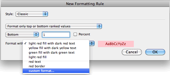
Then select Format only top or bottom ranked values in the first drop down, Bottom in the second drop down and enter 1 in the final box. In our example, we've selected only the first bottom value.

Next, we need to select what formatting to apply when this second condition is met. To do this, select custom format from the Format with drop down.

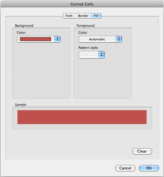
When the Format Cells window appears, select the Fill tab. Then select the color that you'd like to see for the lowest value in the range. In this example, we've selected red. We also went to the Font tab and set the Color to Automatic.

Then click on the OK button.

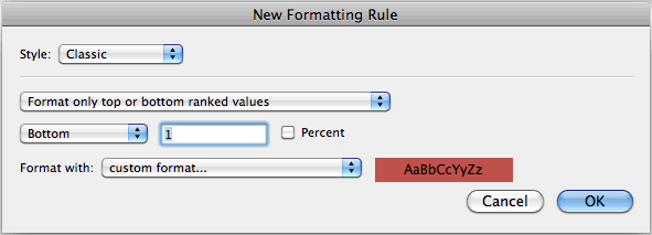
When you return to the New Formatting Rule window, you should see the preview of the formatting in the Preview box. In this example, the preview box shows red as the fill color. Next click on the OK button.

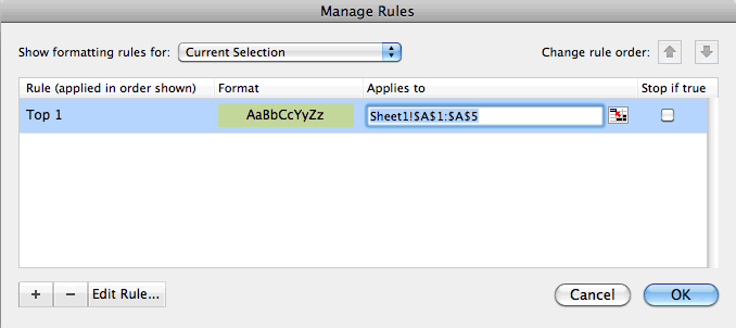
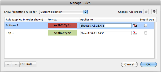
Your Manage Rule window should now look like this.

Click on the OK button.

Now when you return to the spreadsheet, the conditional formatting will be applied. As you can see, the -3 value appears in a red cell while the 200 value appears in a green cell.