

MS Excel: Frequently Asked Questions for VLOOKUP Function
Interested in learning more about the VLOOKUP function? Here are some questions that others have asked about the VLOOKUP function.
Frequently Asked Questions
Question: In Microsoft Excel, I'm using the VLOOKUP function to return a value. I want to sum the results of the VLOOKUP, but I can't because the VLOOKUP returns a #N/A error if no match is found. How can I sum the results when there are instances of #N/A in it?
Answer: To perform mathematical operations on your VLOOKUP results, you need to replace the #N/A error with a 0 value (or something similar). This can be done with a formula that utilizes a combination of the VLOOKUP function, IF function, and ISNA function.
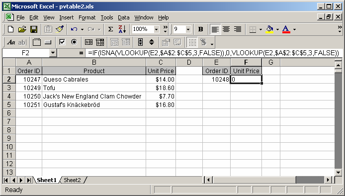
Based on the spreadsheet above:
=IF(ISNA(VLOOKUP(E2,$A$2:$C$5,3,FALSE)), 0, VLOOKUP(E2,$A$2:$C$5,3,FALSE))
Result: 0
First, you need to enter a FALSE in the last parameter of the VLOOKUP function. This will ensure that the VLOOKUP will test for an exact match.
If the VLOOKUP function does not find an exact match, it will return the #N/A error. By using the IF and ISNA functions, you can return the Unit Price value if an exact match is found. Otherwise, a 0 value is returned. This allows you to perform mathematical operations on your VLOOKUP results.
Question: I have a list of #s in column A (lets say 1-20). There is a master list in another column that may not include some of the column A #s. I want a formula in column B to say (if A1 exists in the master list, then "Yes", "No"). Is this possible?
Answer: This can be done with a formula that utilizes a combination of the VLOOKUP function, IF function, and ISNA function.
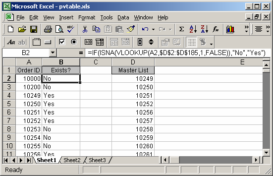
Based on the spreadsheet above:
=IF(ISNA(VLOOKUP(A2,$D$2:$D$185,1,FALSE)), "No", "Yes")
Result: "No"

=IF(ISNA(VLOOKUP(A5,$D$2:$D$185,1,FALSE)), "No", "Yes")
Result: "Yes"
First, you need to enter a FALSE in the last parameter of the VLOOKUP function. This will ensure that the VLOOKUP will test for an exact match.
If the VLOOKUP function does not find an exact match, it will return the #N/A error. By using the IF and ISNA functions, you can return a "Yes" value if an exact match is found. Otherwise, a "No" value is returned.
Question: To automate a spreadsheet: I am trying to write a formula using a Lookup formula in F14 so that when a rock type (say sh for shale) is entered in D14 it will look up the rock type in Q1 thru Q10 and fill in F14 with cell format fill pattern from S1 thru S10. How do I get it to recognize the format pattern and copy it to F14?
Answer: You can do this with a VLOOKUP function as follows:
=VLOOKUP(D14, $Q$1:$S$10, 3, FALSE)
In this VLOOKUP example, the rock type that you want to look up is in cell D14, the lookup data is found in the range of $Q$1:$S$10. We've absolutely referenced the lookup range so that you can copy the formula to other cells without the range changing. The third parameter is set to 3 because we want the value returned from column S which is the third column in the range of $Q$1:$S$10. And the final parameter in the VLOOKUP is FALSE because we are only looking for an exact match.
With this formula if a match is not found, the VLOOKUP will return #N/A. If you would like to return a different value when there is no match, say "Not Found", then you could modify your VLOOKUP as follows:
=IF(ISNA(VLOOKUP(D14, $Q$1:$S$10, 3, FALSE)), "Not Found", VLOOKUP(D14, $Q$1:$S$10, 3, FALSE))
This formula would return "Not Found" if there was not a match. Otherwise, it would return the appropriate value from S1 to S10.
Question:I want to do a VLOOKUP if a statement is true.
Example:
If cell A2 = cell F9, I want to do a virtual lookup depending on what is in cell E34, the function would return corresponding data from cells defined as "TEAM".
This is what I came up with:
=If(A2=F9),VLOOKUP(+E34,TEAM,1+1)
Answer: You are very close. Since we don't know how many columns are in your named range called "TEAM", we'll just assume that you want to return corresponding data from the second column in "TEAM". As such, you can do this with the VLOOKUP formula as follows:
=IF(A2=F9,VLOOKUP(E34,TEAM,2,FALSE))
In this example, VLOOKUP will be performed only if A2 is equal to F9.
The first parameter of E34 specifies the value to lookup. The second parameter uses the named range called "TEAM" which is where the lookup data is found. The third parameter of 2 will return corresponding data from the second column in the "TEAM" named range. The final parameter of FALSE means that we are only looking for an exact match.
Advertisements