---

MS Excel 2010: Change the fill color of a cell based on the value of an adjacent cell

This Excel tutorial explains how to use conditional formatting to change the fill color of a cell based on the value of another cell in Excel 2010 (with screenshots and step-by-step instructions).

Question: In Microsoft Excel 2010, I'm trying to apply a fill color to a cell based on the value in an adjacent cell. How can I do this?

Answer: If you wish to change the fill color in a cell based on the value of an adjacent cell, you will need to apply conditional formatting.

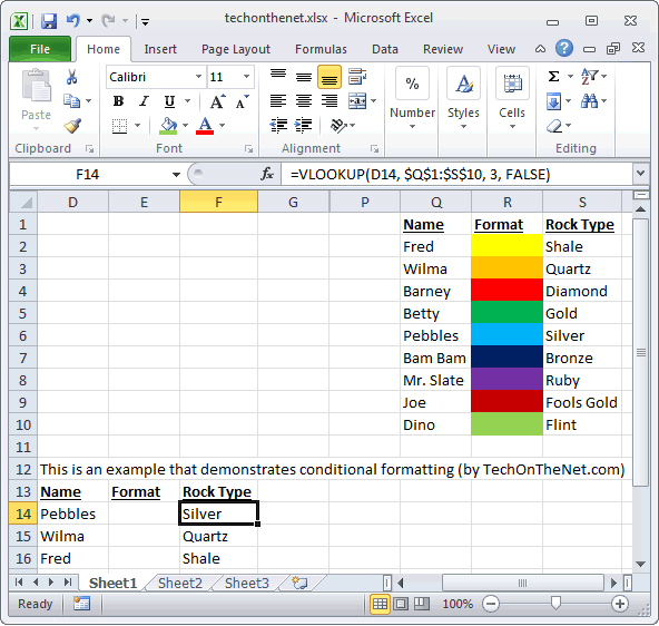
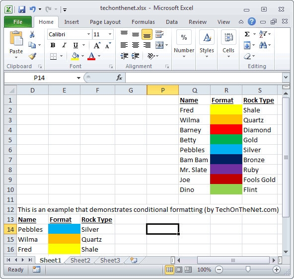
In this example, we have a table in cells Q1 to S10 that display the fill colors that we want to apply for each rock type. So in this example, we want to display a yellow fill color if the Rock Type is Shale, an orange fill color if the Rock Type is Quartz, and so on.

We use a VLOOKUP in cell F14 to F16 to pull the appropriate Rock Type from the Q1:S10 table. Now the hard part. We want to display the corresponding fill color in cells E14 to E16 based on the Rock Type returned. We are unable to use a VLOOKUP to pull the fill color, so we will have to use conditional formatting.

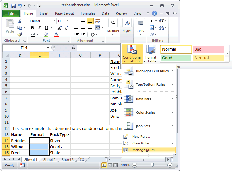
To do this, select the range of cells that you wish to apply the conditional formatting to. In this example, we've selected cells E14 to E16. Then select the Home tab in the toolbar at the top of the screen. Then in the Styles group, click on the Conditional Formatting drop-down and select Manage Rules.

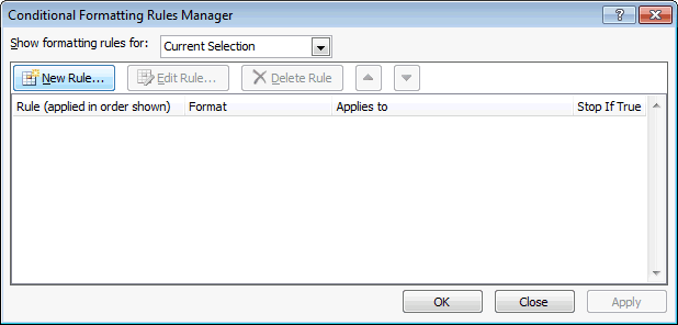
When the Conditional Formatting Rules Manager window appears, click on the "New Rule" button to enter the first condition.

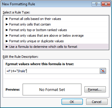
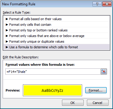
When the New Formatting Rule window appears, select Use a formula to determine which cells to format as the rule type.

Then type the following formula:

=F14="Shale"

Next, we need to select what formatting to apply when this condition is met. To do this, click on the Format button.

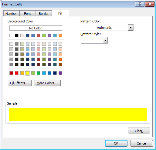
When the Format Cells window appears, select the formatting conditions that you wish to apply. In this example, we've selected yellow as the Fill Color. Then click on the OK button.

When you return to the New Formatting Rule window, you should see the preview of the formatting in the Preview box. In this example, the preview box shows the fill color of yellow. Next click on the OK button.

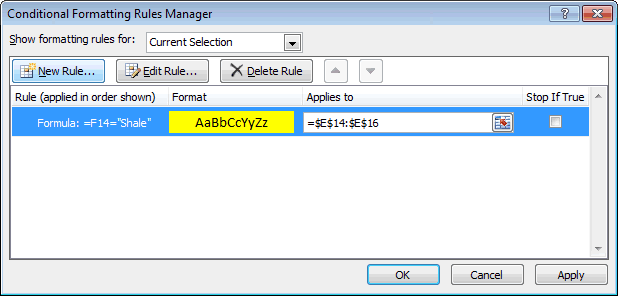
This will return you to the Conditional Formatting Rules Manager window. You can now view the first conditional formatting condition. We will need to add a condition for each fill color by clicking on the New Rule button and repeating the previous steps.

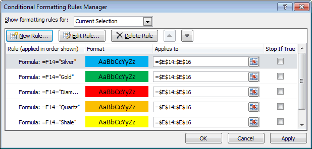
Once all of the conditions have been entered, you should see something like the picture below. Click on the OK button.

Now when you return to the spreadsheet, the conditional formatting will be applied in cells E14 to E16.