---

MS Excel 2003: Highlight 1st, 2nd, 3rd highest scores

This Excel tutorial explains how to use conditional formatting to highlight the first, second, and third highest values in Excel 2003 and older versions (with screenshots and step-by-step instructions).

Question: In Microsoft Excel 2003/XP/2000/97, how can I apply conditional formatting to highlight the 1st, 2nd, and 3rd highest scores in a different color?

Answer: To do this, first highlight the cells that you wish to apply the formatting to. In this example, we've selected cells E6 to E15 in the spreadsheet. Then select Conditional Formatting under the Format menu.

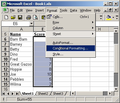
When the Conditional Formatting window appears, select "Cell Value Is" in the first drop down and "equal to" in the second drop down. Then enter the following formula that uses the LARGE function:

=LARGE($E$6:$E$15,1)

This formula uses the LARGE function to return the highest value from cells E6 to E15.

Next, we need to select the color we want to use to shade the highest score. To do this, click on the Format button.

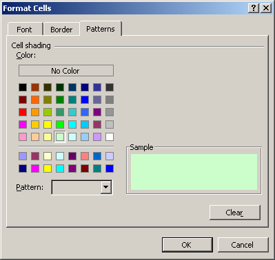
When the Format Cells window appears, select the Patterns tab. Then select the color that you'd like to see. In this example, we've selected a light green. Then click on the OK button.

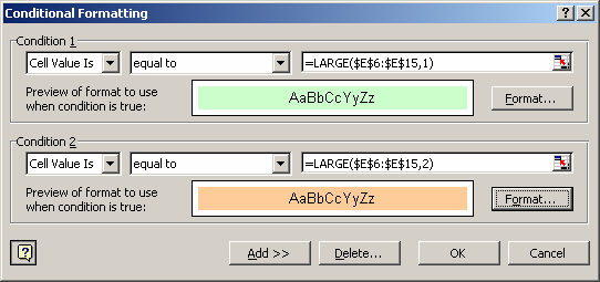
When you return to the Conditional Formatting window, you should see the following. Next, click on the Add button.

You should now see a Condition 2. Again select "Cell Value Is" in the first drop down and "equal to" in the second drop down. Then enter the following formula:

=LARGE($E$6:$E$15,2)

This formula will return the 2nd highest value from cells E5 to E15. Click on the Format button and select the formatting that you'd like to apply to the 2nd highest score. In this example, we've selected an orange pattern.

Click on the Add button one more time.

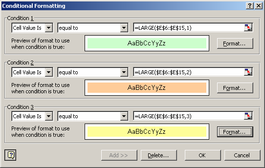
You should now see a Condition 3. Again select "Cell Value Is" in the first drop down and "equal to" in the second drop down. Then enter the following formula:

=LARGE($E$6:$E$15,3)

This formula will return the 3rd highest value from cells E5 to E15. Click on the Format button and select the formatting that you'd like to apply to the 3nd highest score. In this example, we've selected a yellow pattern.

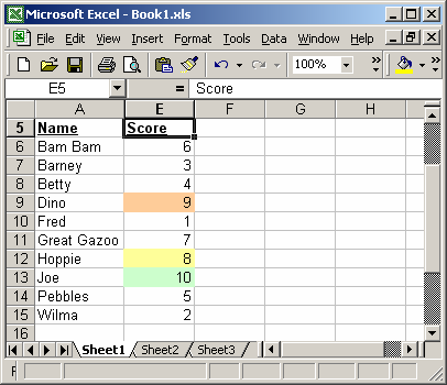
Now when you return to the spreadsheet, the conditional formatting will be applied.

As you can see, the 1st highest score is highlighted in green, the 2nd highest score is highlighted in orange, and the 3rd score is highlighted in yellow.