---

MS Excel 2007: Automatically alternate row colors (three shaded, three white)

This Excel tutorial explains how to use conditional formatting to automatically alternate row colors, three shaded and three white, in Excel 2007 (with screenshots and step-by-step instructions).

Question: How can I set up alternating row colors in Microsoft Excel 2007? I want to alternate between 3 shaded rows and 3 white rows.

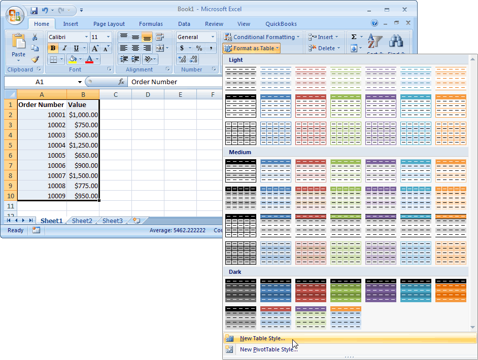
Answer: To do this, first highlight the rows that you wish to apply the formatting to. In this example, we've selected cells A1:B10.

Select the Home tab in the toolbar at the top of the screen. Then in the Styles group, click on the Format as Table drop-down and select New Table Style at the bottom of the list.

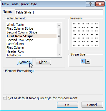
When the New Table Quick Style window appears, select First Row Stripe as the Table Element. Then change the Stripe Size to 3. Click on the Format button.

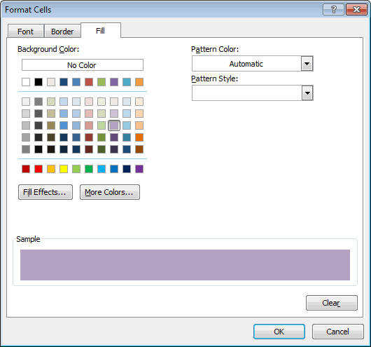
Click on the Fill tab and select the color for the shaded rows. In this example, we have selected a purple. Click the OK button.

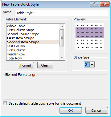
select Second Row Stripe as the Table Element. Then change the Stripe Size to 3. Click the OK button.

When you return to the spreadsheet, click on the Format as Table drop-down in the Styles group again and select the new customized style that you just created. It will appear in the top row under Custom.

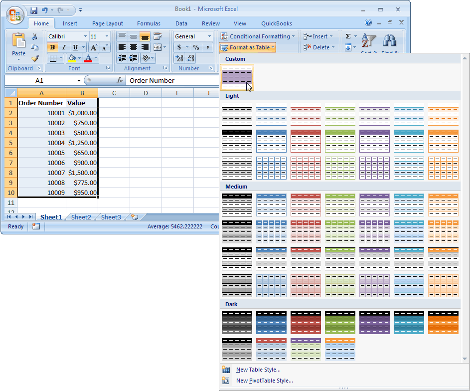
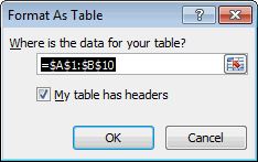
The Format as Table window will pop-up for you to confirm the cell range that will be formatted and the option for you to apply the format to the header rows (ie: My table has headers). Click the OK button to apply the format.

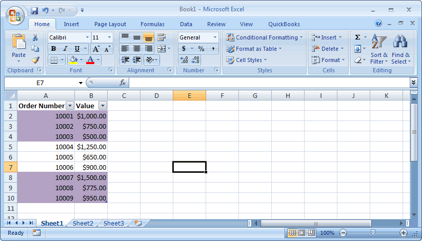
As you can see, you now have alternating colors - 3 shaded rows followed by 3 white rows. You can insert, delete, and move rows, and you don't have to worry about reapplying formatting.