---

MS Excel 2007: Automatically highlight expired dates and dates that are 30 days from expiration

This Excel tutorial explains how to use conditional formatting to automatically highlight expired dates and dates that are 30 days from expiration in Excel 2007 (with screenshots and step-by-step instructions).

Question: In Microsoft Excel 2007, is there a way to automatically highlight upcoming and past due dates?

For example, I have dates that certificates will expire in a spreadsheet. I would like Excel to highlight the ones that are 30 days from expiration in yellow and the ones that are past the expiration in red. Is that possible?

Answer: Yes, you can use conditional formatting to achieve exactly what you are looking for.

First highlight the range of cells that you want to apply the formatting to. In this example, we've selected all of column A since we don't know how many rows will have expiration date values.

Select the Home tab in the toolbar at the top of the screen. Then in the Styles group, click on the Conditional Formatting drop-down and select Manage Rules.

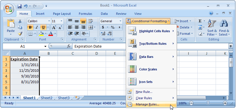
When the Conditional Formatting Rules Manager window appears, click on the "New Rule" button to enter the first condition.

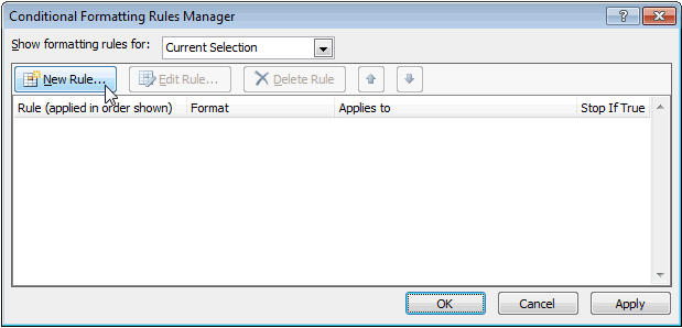
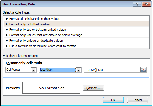
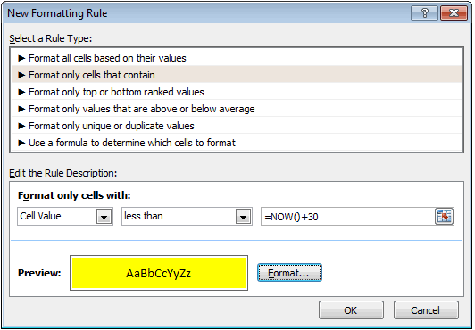
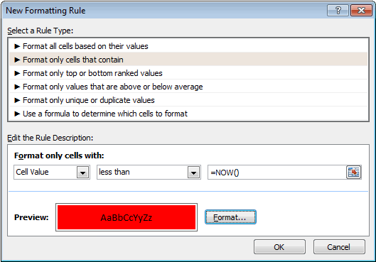
When the New Formatting Rule window appears, select Format only cells that contain as the rule type.

Then select Cell Value in the first drop down, less than in the second drop down, and enter the following formula that uses the NOW function:

=NOW()+30

Next, we need to select what formatting to apply when this condition is met. To do this, click on the Format button.

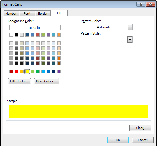
When the Format Cells window appears, select the Fill tab. Then select the color that you'd like to see the dates that will expire in the next 30 days. In this example, we've selected yellow. Then click on the OK button.

When you return to the New Formatting Rule window, you should see the preview of the formatting in the Preview box. In this example, the preview box shows yellow as the fill color. Next click on the OK button.

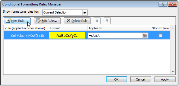
This will return you to the Conditional Formatting Rules Manager window.

You will need to click on the New Rule button again.

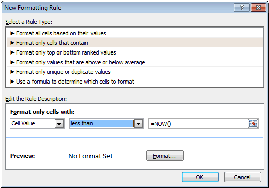
When the New Formatting Rule window appears, select Format only cells that contain as the rule type.

Then select Cell Value in the first drop down, less than in the second drop down, and enter the following formula that uses the NOW function:

=NOW()

What this formula means is that the date in the cell is past today's date. To select what formatting to apply when this condition is met. To do this, click on the Format button.

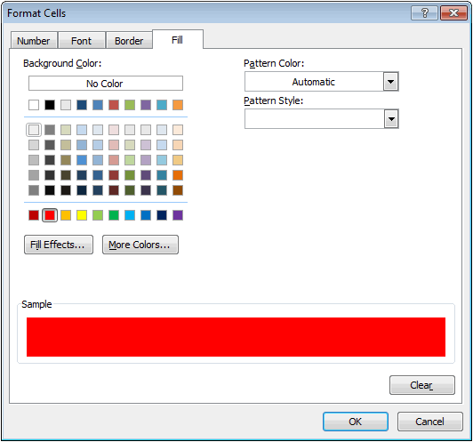
When the Format Cells window appears, select the Fill tab. Then select the color that you'd like to see the expired dates displayed in. In this example, we've selected red. Then click on the OK button.

When you return to the New Formatting Rule window, you should see the preview of the formatting in the Preview box. In this example, the preview box shows red as the fill color. Next click on the OK button.

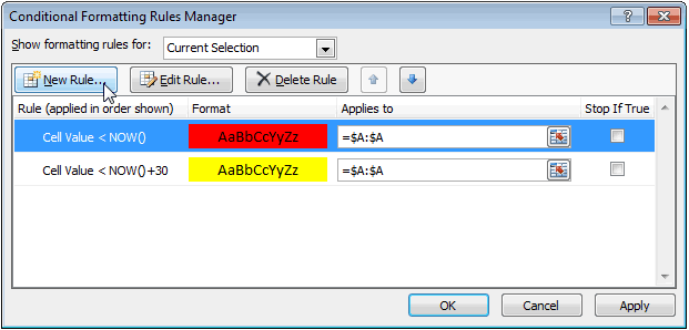
This will return you to the Conditional Formatting Rules Manager window.

You will need to click on the New Rule button again.

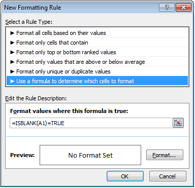
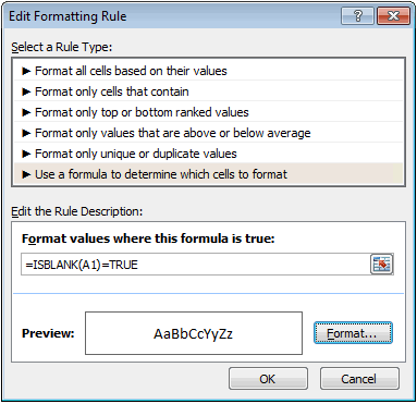
When the New Formatting Rule window appears, select Use a formula to determine which cells to format as the rule type.

Then enter the following formula that uses the ISBLANK function:

=ISBLANK(A1)=TRUE

What this formula means is that if any cells in column A are blank, do not apply the yellow or red formatting. The value of A1 is put as the parameter in the ISBLANK function since this is the first value in the range of cells that you've selected. Since the formula uses relative referencing each value in column A will be evaluated individually.

Next, we need to select what formatting to apply when this condition is met. To do this, click on the Format button.

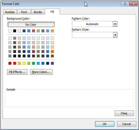
When the Format Cells window appears, select the Fill tab. Then select white as the color that you'd like to see as the fill in the blank cells. Then click on the OK button.

When you return to the New Formatting Rule window, you should see the preview of the formatting in the Preview box. In this example, the preview box shows white as the fill color. Next click on the OK button.

Now when you return to the Conditional Formatting Rules Manager window, make sure that you check the "Stop If True" checkbox for the first rule. If you do not, the blank cells will show as red fill because the second condition will also evaluate as TRUE.

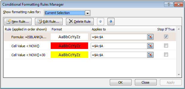
Click on the OK button.

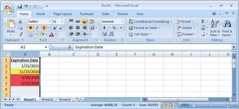
Now when you return to the spreadsheet, the conditional formatting will be applied.

Since we created this example on 11/19/2010, you can see that the value in cell A3 will expire in the next 30 days, while the value in cells A4 and A5 have already expired.