

MS Excel 2003: Use an array formula to perform a two criteria lookup
This Excel tutorial explains how to use an array formula to perform a two criteria lookup in Excel 2003 and older versions (with screenshots and step-by-step instructions).
Question: I have the following table in Microsoft Excel 2003/XP/2000/97:
| Column A | Column B | Column C | Column D | Column E |
|---|---|---|---|---|
| EL_ID | LD_ID | nx | ny | qxy |
| 3000 | L001 | -10.8 | -280.9 | 981.0 |
| 3000 | L002 | -145.0 | -315.0 | 441.1 |
| 3000 | L003 | -122.2 | -315.8 | 451.2 |
| 3001 | L001 | -6.4 | -135.6 | -161.8 |
| 3001 | L002 | -8.2 | -154.0 | -157.9 |
| 3001 | L003 | -8.3 | -154.7 | -167.9 |
I’m trying to create a formula in Excel that returns the corresponding qxy value, given a EL_ID and LD_ID value.
For example, I need the formula to return a qxy value of -161.8, given an EL_ID=3001 and LD_ID="L001".
How can I do this?
Answer: This can be done in Excel with an array formula.
Let's look at an example.

In cell A10, we've created the following array formula that uses the INDEX, MATCH and IF functions:
=INDEX(E2:E7,MATCH(3001,IF(B2:B7="L001",A2:A7),0))
When creating your array formula, you need to use Ctrl+Shift+Enter instead of Enter. This creates {} brackets around your formula as follows:
{=INDEX(E2:E7,MATCH(3001,IF(B2:B7="L001",A2:A7),0))}
What this formula does is perform a two criteria lookup. It looks for a value of 3001 in cells A2:A7 and "L001" in cells B2:B7, and returns the corresponding value from column E (ie: E2:E7). In this example, it returns a value of -161.8 from column E.
If you wanted to instead lookup an EL_ID=3000 and LD_ID=L003, as in this example:
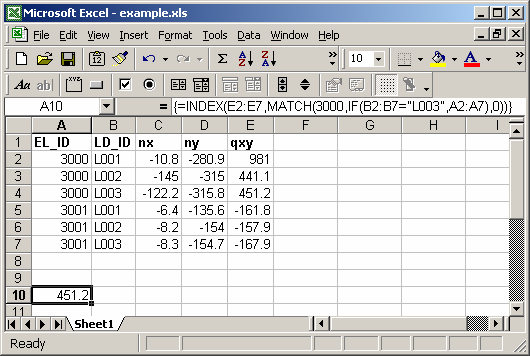
In cell A10, we've created the following array formula:
=INDEX(E2:E7,MATCH(3000,IF(B2:B7="L003",A2:A7),0))
When creating your array formula, you need to use Ctrl+Shift+Enter instead of Enter. This creates {} brackets around your formula as follows:
{=INDEX(E2:E7,MATCH(3000,IF(B2:B7="L003",A2:A7),0))}
What this formula does is perform a two criteria lookup. It looks for a value of 3000 in cells A2:A7 and "L003" in cells B2:B7, and returns the corresponding value from column E (ie: E2:E7). In this example, it returns a value of 451.2 from column E.
Advertisements