---

MS Excel 2013: How to Handle Errors in a Pivot Table

This Excel tutorial explains how to change the display of errors in a pivot table in Excel 2013 (with screenshots and step-by-step instructions).

Question: In Microsoft Excel 2013, I don't want to see errors in the pivot table. How do I replace all errors with another value?

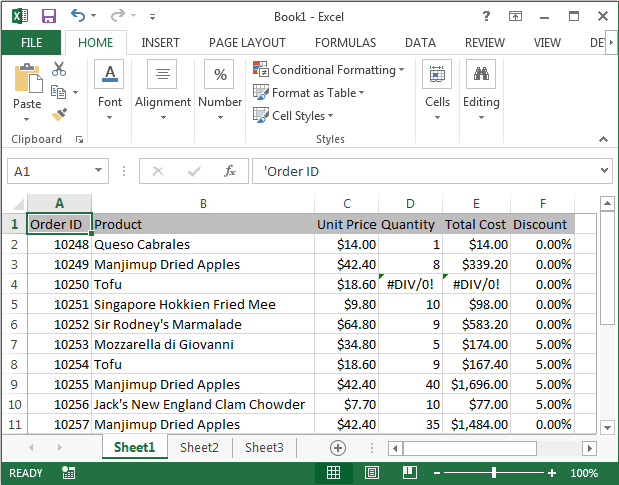
Answer: Let's first take a look at an example of an error in a pivot table. This is a picture of our underlying data for the pivot table. You can see in row 4 that the quantity entry has an error in it. This could be the result of a mathematical formula, for example.

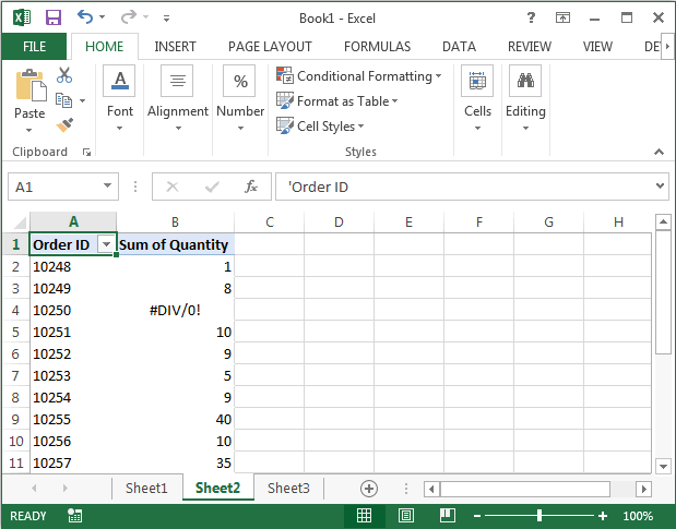
Now when you take a look at the pivot table that uses this data, you can see the error in the pivot table.

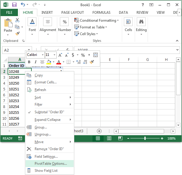
You can replace this error with a more appropriate value. To do this, right-click on the pivot table and then select "PivotTable Options" from the popup menu.

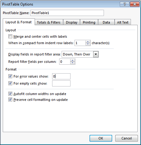
When the PivotTable Options window appears, check the checkbox called "For error values show". Then enter the value that you wish to see in the pivot table instead of the error. Click on the OK button. In this example, we've decided to replace the error with a 0.

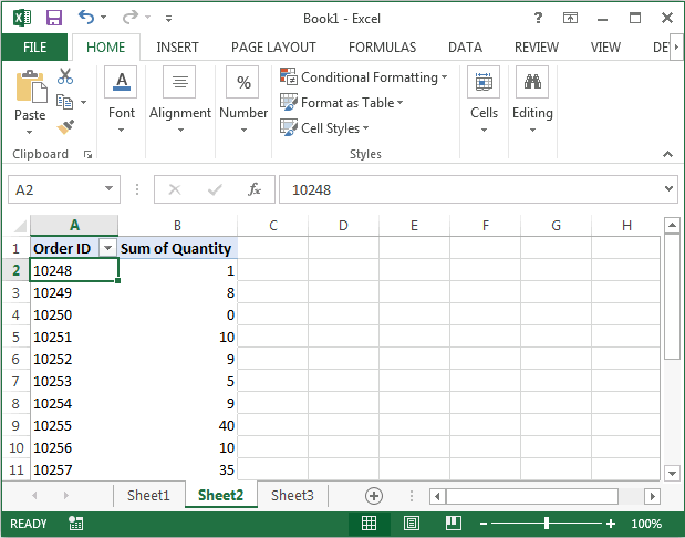
Now when we return to the pivot table, this is what we'll see. The error value has now been replaced with 0.